Hardness Variability Benchmarking

Benchmarking the hardness of a particular ore deposit can provide valuable intelligence as to whether its comminution properties are typical of other deposits and if not, the extent to which they are likely to depart from the norm.  Such information may be useful in the early investigative and developmental stages of a prospective ore deposit as it provides an indication as to whether the likely comminution energy requirement, the cost of which is often a major economic factor, will be more or less the same as that of existing concentrators.  In such a benchmarking exercise the most relevant and hence useful comparison will be between the hardness data of the prospective deposit and existing deposits with the same valuable mineral content (referred to as “commodity”) and geographical location. To do so a large database is required.  SMC Testing has such a database which is arguably the largest and most detailed of its kind in the world.  As at December 2019 the database numbered over 50,000 results from hardness testing of over 1900 deposits using the SMC Test^®. Each test generates a range of parameters which can be used for comminution circuit simulation and predicting comminution circuit specific energy.  These are detailed in Table 1.  There a total of 10 which, when combined with geographical location and commodity data means that the database contains upwards of 700,000 data points.

Table 1 – SMC Test parameter Outputs and Their Uses

Commodities and Locations

The database has results covering 49 different commodities.  In many cases ore deposits produce more than one commodity eg copper/gold, lead/zinc etc.  In such cases test results have been categorised in terms of the commodity that the owner of the deposit has reported as being the principal one.  A list of the different commodities is given in Table 2, whilst Figure 1 shows how the 50,000 SMC Tests in the data base are distributed amongst them.  As can be seen, Copper and Gold predominate, accounting for just over 80%.  Figure 2 shows how the deposits are distributed.  This distribution is quite different and reflects the fact that copper mining companies tend to carry out many more SMC Test per deposit and is due to the fact that geometallurgical modelling, which requires relatively large numbers of ore characterisation tests, is more common amongst such mines.

Table 2 – List of Commodities Covered by the SMC Test Database

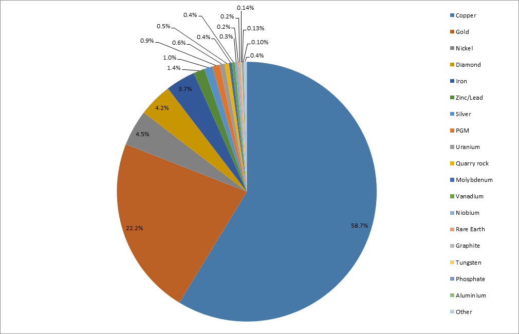
Figure 1 - Distribution of 50,000 Global SMC Tests by Principal Commodity

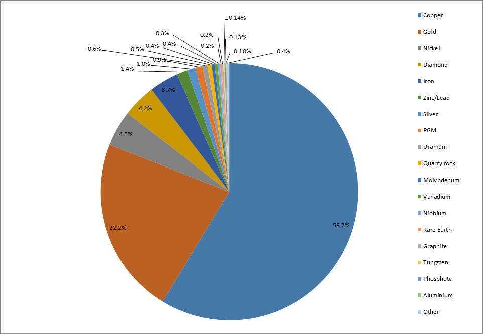
Figure 2 - Distribution of 1900 Global Ore Deposits in SMC Test Database by Principal Commodity

In terms of location the test results have been organised into country of origin of which almost 100 are covered.  These are listed in Table 3. Figure 3 shows how the 50,000 SMC Tests in the database are distributed amongst the continents they are in, whilst Figure 4 shows the distribution in terms of deposits.  There are marked differences in the distributions based on deposits and number of SMC Tests, particularly for Central and South America.  This reflects the far more widespread use of geometallurgical modelling, which when done well, requires relatively large numbers of ore characterisation tests, such as SMC Tests.  Hence on average it is found that the number of SMC Tests per deposit is significantly higher in this region than anywhere else in the world.

Table 3 – List of Countries Covered by the SMC Test Database

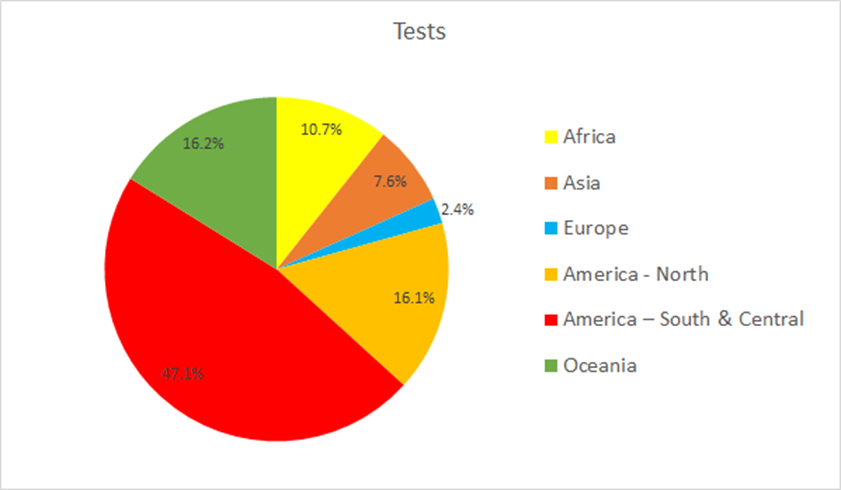
Figure 3 - Distribution of 50,000 Global SMC Tests in Database by Continent

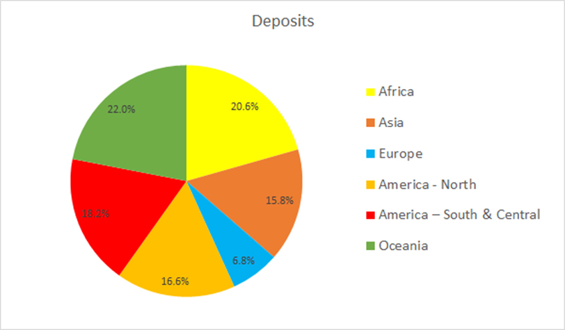
Figure 4 - Distribution of 1900 Global Ore Deposits in SMC Test Database by Continent

Analysis

The data base gives a unique insight into how the hardness of the world’s orebodies varies.  For the purposes of this paper the DWi will be used to illustrate the nature of this variation.

Looking at the database as a whole gives a mean DWi of 6.69 kWh/m³, minimum and maximum values being 0.06 and 21.9 kWh/m³ respectively. A histogram of the DWi values is shown in Figure 5, whilst the associated cumulative distribution is given in Figure 6.  Analysis shows the data to be normally distributed. 

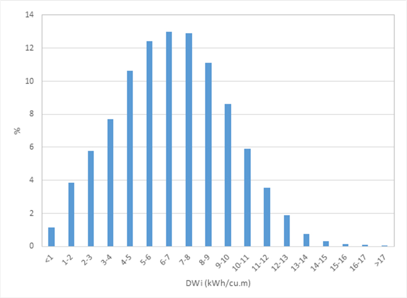
Figure 5 – Histogram of DWi Values Worldwide

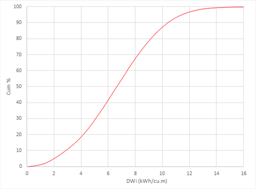
Figure 6 – Cumulative Distribution of DWi Values Worldwide

The sg of an ore is often overlooked by minerals processors and whilst it does not convey any direct indication of rock strength, changes in its value within and between ore bodies indicates changes in the nature of the rock that sometimes does correlate with hardness changes.   The database mean value is 2.79, whilst minimum and maximum values are 1.35 and 4.91 respectively. A histogram of the distribution of sg values is shown in Figure 7.

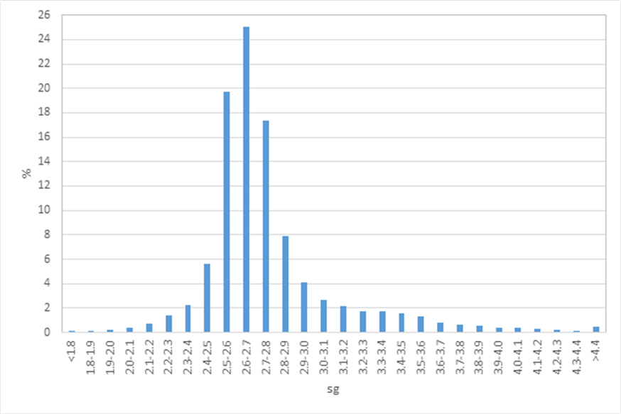
Figure 7 – Histogram of SG Values Worldwide

Looking at how strength varies with commodity in the world’s ore deposits it is seen that mean values vary widely as Figure 8 indicates.  The associated sg values, which are shown in Figure 9 similarly also vary widely.

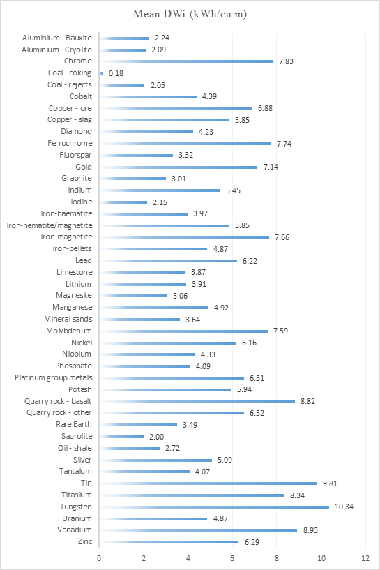
Figure 8 – Variation in Mean DWi Value with Ore Commodity

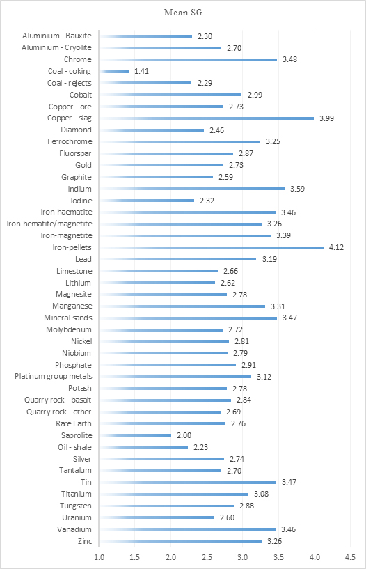
Figure 9 – Variation in Mean SG Value with Ore Commodity

Mean strength of deposits when viewed at a continental level shows relatively little variation as Table 4 illustrates.  This may be as expected as these values are dictated by the mix of commodities in each continent which tends to be quite similar.

Table 4 – Variation in Mean DWi Value with Continental Location