A New Autogenous and Semi-autogenous Mill Model For Scale-up, Design and Optimisation

S.Morrell SMCC Pty Ltd

E-mail: This email address is being protected from spambots. You need JavaScript enabled to view it.

ABSTRACT

The successful application of modelling and simulation in design and optimisation rests heavily on having a model which is lifelike. In the case of Autogenous (AG) and Semi-autogenous (SAG) mills this has provided a significant challenge to modellers, due in part to the interaction between feed characteristics and mill performance and also due to the difficulty in obtaining high quality relevant data from full-scale circuits. As a result the literature contains numerous papers on AG/SAG mill modelling, the majority of which contain little or no data to indicate how well the models predict full-scale mill performance. In an attempt to address this problem a new AG/SAG mill model has been developed which incorporates the capability to respond to changes in most design and operational variables. The model can be used as a stand-alone design tool, to scale-up from pilot data and to optimise existing circuits. It predicts throughput, power draw and product size distribution as well as load size distributions and slurry hold-up. The overall structure of the model and the sub-processes that it contains is described. The model is successfully validated using data from over 21 different full-scale circuits.

INTRODUCTION

Modelling and simulation of autogenous (AG) and semi-autogenous (SAG) mills are valuable tools for helping to design the best circuit for a given application and subsequently to optimise its performance. This can be achieved by narrowing the choice of the most likely successful processing routes at the pre-feasibility stage, as well as augmenting a pilot test programme with simulations using breakage characterisation data from drill core samples. In cases where pilot-scale testwork is not possible, simulations using models which are based on data from a wide range of full scale circuits can significantly reduce the risk of not piloting. Even where pilot data are available simulations using data from a database, where a good match can be made in terms of ore hardness and circuit design, provides an additional and very valuable crosscheck against the pilot results. Added advantages of the simulation route are its versatility, its ability to simulate the entire comminution circuit and the ease with which combinations of circuit designs can be evaluated on a throughput, power draw and product size basis. Perhaps its most important advantage over the more traditional power-based techniques is its ability to interface with blast fragmentation models so as to assess and optimise the impact of blast design and ROM feed size distribution. Practical experience has shown that feed size variation can be significant and this can have a major impact on AG and SAG mill circuit performance.

The successful application of modelling and simulation in design and optimisation rests heavily on having a model which is lifelike. In the case of AG and SAG mills this has provided a significant challenge to modellers, due in part to the interaction between feed characteristics and mill performance and also due to the difficulty in obtaining high quality relevant data from full-scale circuits. As a result the literature contains numerous papers on AG/SAG mill modelling, the majority of which contain little or no data to indicate how well they predict full scale mill performance (Austin et al, 1976, 1985, 1987, Barahona, 1984, Nordell et al, 2001, Weymont, 1979). Stanley's work (1974) and that of Leung over a decade later (1987) stand out in that both researchers went to great lengths to obtain pilot and full-scale mill data with which to indicate how well their models predicted observed data. However, the range of mills they studied was limited and although their data are very useful they cover a relatively small part of the spectrum of designs currently seen in operating plants around the world. In an attempt to address this problem a new AG/SAG mill model has been developed which incorporates the capability to respond to changes in most design and operational variables and which has been validated using a wide range of industrial data.

MODEL DEVELOPMENT

Introduction

In grinding mills the energy that the rotation of the mill shell imparts to the grinding media is subsequently transferred to ore particles with which they are in contact, so causing breakage. The process is a discrete one, as it comprises many individual collisions or breakage "events". The products of these breakage events may then leave the mill via the discharge grates and pulp lifters due to entrainment by slurry, or remain to undergo further breakage. The specific energy associated with particle breakage is related to the energy of the grinding media and the mass of the target rocks, whilst the frequency of these events is associated with the number of grinding media and the rate at which they circulate within the mill. Hence for modelling purposes it is necessary to have a description of at least the following:

• frequency of breakage events for each size fraction
• energy associated with each breakage event
• size distribution of the products from each breakage event
• transport of slurry through the grates/pulp lifter

The above sub-processes are all related to the size reduction, throughput and power response of the mill and hence, by suitably configuring the model, all three characteristics can be simultaneously predicted from the one overall model.

Size Reduction and Throughput

The most useful framework for encapsulating the size reduction process in a grinding mill is one based on the so-called population balance model (Epstein, 1947), the Whiten variant of this approach (1974) being the most valuable for AG/SAG mill modelling. The model contains two equations:

$$ 0 = f_i + p_i + \sum_{i=1}^{i} r_j s_j a_{ij} - r_i s_j $$ (1)

where,

\( f_i \) = tph of particles of size i in the feed

p_i = tph of particles of size i in the product

\( r_i \) = breakage rate of particles of size i

\( s_i \) = mass of particles in the charge of size i

\( d_i \) = discharge rate of particles of size i

a_ii = breakage distribution function

The simplicity of this model is both the source of its greatest strengths and greatest weaknesses. Its greatest strengths are its ease of use and great versatility, whilst its greatest weakness is the lack of any physical description of the sub-processes on which it depends. For it to be used successfully, therefore, a series of supplementary models must be developed and linked to it. These are described in the following sections.

Transport

Transport of slurry out of the mill is described using a discharge function, which by rearranging equation 2 can be defined as:

For a given mill the values of \( d_i \) can be calculated from measurements of the mass and size distribution of rocks in the mill \( (s_i) \) , and the throughput and the size distribution of rocks exiting the mill \( (p_i) \) . However, measuring the size distribution and mass of rocks in a full-scale mill is extremely difficult and hence much of the data that are available on the shape of the discharge function relate to the pilot scale (Stanley, 1974, Leung, 1987). Very few data have been reported on full-scale mills (Stanley, 1974, Morrell, 1989) but these confirm the shape of the function seen at the pilot scale. By way of example raw data from a 7m SAG mill are given in Figure 1. The function is characterised by two regions. The first extends up to a particle size of about 1mm \( (x_m) \) , where the discharge rate is largely constant and equal to that of water. Therefore particles smaller than 1mm plus their associated water are assumed to behave as an homogenous fluid. For particles above about 1mm the discharge rate progressively reduces and reflects their increasing tendency to be influenced by the classifying action of the grate. As a result the function reaches zero at a particle size near to the grate/pebble port aperture, which in this case was 18mm.

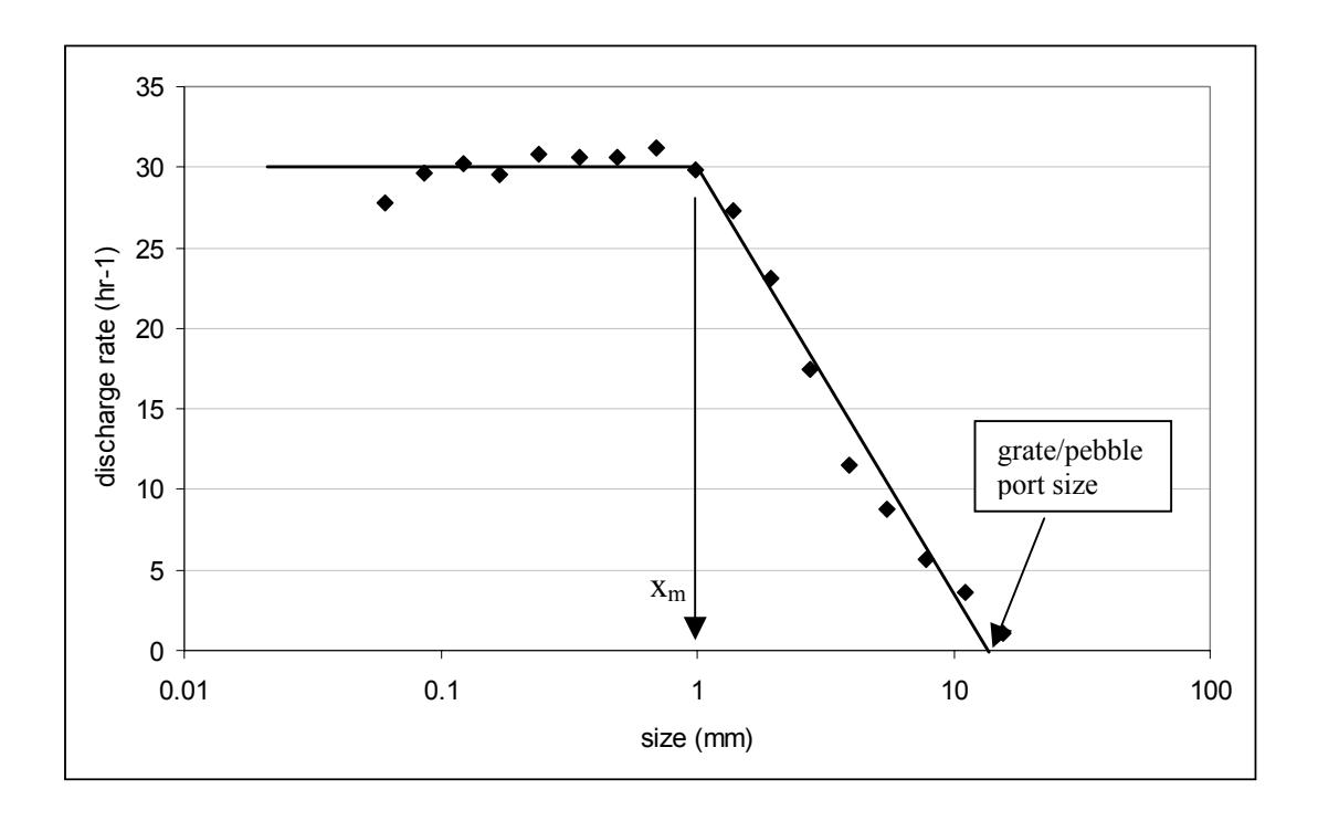
To model the discharge function advantage was taken of the two distinct regions illustrated in Figure 1. The region with a constant discharge rate reflects the purely fluid characteristics of the discharge stream. This constant rate \( (d_m) \) is directly related to the slurry flow rate out of the mill and the quantity held up in the mill itself. This is seen from equation 3, which for water and particles smaller than \( x_m \) can be re-written as:

The summations in the numerator and denominator in equation 4 are the slurry discharge and hold-up respectively, where slurry is defined as water plus all particles smaller than \( x_m \) . Hence, to determine \( d_m \) an equation relating slurry hold-up in a mill to the rate at which it flows out is required. Such a model was constructed using the approach originally adopted by Morrell and Stephenson (1996). In this approach two equations were developed, one of which related to flow via the grinding charge interstices and the other to flow via the slurry pool, in cases where this was present. Morrell and Stephenson incorporated the effects of grate design, mill speed and charge volume. However, the range of grate designs they used for their experimental programme was very limited and, more seriously, did not take into account the effect of pulp lifters. Latchireddi (2002) rectified this deficiency by conducting a detailed laboratory and pilot study of the influence of grate design and pulp lifters. His results were then used to revise the original equations and incorporate the influence of pulp lifter depth ( \( \lambda \) ). The result was the following general equation:

$$ J_{s} = \eta \gamma^{n_{1}} A^{n_{2}} J_{t}^{n_{3}} \phi^{n_{4}} Q^{n_{5}} D^{n_{5}} $$ $$ \tag{5} $$

where,

\( J_s \) = the net fractional slurry hold-up inside the mill

A = fractional open area

\( J_t \) = fractional grinding media volume

\( \phi \) = fraction of critical speed

Q = slurry discharge flowrate

\( \gamma \) = mean relative radial position of the grate holes

\( \eta \) = coefficient of resistance which varied depending on whether flow was

via the grinding media interstices or the slurry pool (where present).

\( n_1 \) - \( n_6 \) = model parameters

The value of \( \gamma \) is a weighted radial position, which is expressed as a fraction of the mill radius and is calculated using the formula:

where,

\( a_i \) = open area of all holes at a radial position \( r_i \)

\( r_m \) = radius of mill inside the liners

The parameter values \( n_1 \) - \( n_6 \) and \( \eta \) were found to be functions of pulp lifter size and were all modelled using the general equation proposed by Latchireddi (2002):

where,

\( n_g \) = parameter values for grate-only condition

\( k_i, k_i = constants \)

\( \lambda \) = depth of the pulp lifter expressed as a fraction of mill diameter

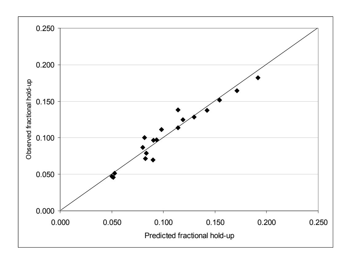
The parameters in the above equations were fitted to over 760 laboratory and pilot mill data sets and 19 full scale mill data sets. The fit of the equations to the full-scale mill data sets are shown in Figure 2.

When analysing the full-scale mill data the discharge slurry flowrate was calculated from the sum of the water plus particles smaller than xm. As a result equation 5 can be directly related to equation 4, which can now be expressed as

Equation 5 is therefore used initially to predict Js from a given slurry flowrate (Q), both Q and Js being subsequently used in equation 8 to predict dm. For most practical purposes xm can be taken to be 1mm and hence for particle sizes up to this size di can be considered to be equal to dm.

Having estimated di for particle sizes up to 1mm the discharge function values for particle sizes greater than 1mm then need to be predicted. This is done using the Leung approach (1987) of using a log-linear relationship, which goes to zero at the grate/pebble port size (see Figure 1).

Breakage Distribution Function

The breakage distribution function is the progeny size distribution that results from breakage of the parent rock. This distribution will vary depending on the rock strength and the energy with which it is broken. The function therefore needs to be ore specific and related to the breakage energy. The JKMRC's approach is ideal for this purpose. This uses a two-parameter description of rock breakage that is obtained from a drop-weight test (Napier-Munn et al, 1996). The two parameters (A and b) are ore specific and relate the t10 (a size distribution index) to the applied specific energy (Ecs). The t10 in turn can be used to generate a full size distribution (Narayanan and Whiten, 1988). The equation used for describing the relationship between the t10 and Ecs is:

$$ t_{10} = A (1 - e^{-b.Ecs}) $$ (9)

The specific comminution energy (Ecs) has the units kWh/t and is the energy applied during impact breakage. As the impact energy is varied, so does the t10. Higher impact energies produce higher values of t10, which are reflected in products with finer size distributions.

Equation 9 provides the means to predict the product size distribution but it requires the specific energy used for breakage before it can predict the t10. Leung's approach is used to do so (Leung, 1987). Leung assumed that, although a wide range of energies are experienced by rocks in a mill, on average it should be linearly related to the mill diameter. He therefore developed an algorithm that estimated the mean grinding media size and calculated its kinetic energy on impact when dropped from a height equal to the mill diameter. The specific energy experienced by each particle size was then estimated using this mean kinetic energy.

Breakage Rate

From equation 1 it can be seen that, providing the feed and product flowrates and size distributions, the mill rock charge mass and size distribution, as well as the breakage distribution function are measured, the breakage rate distribution can be backcalculated. An example of the resultant distribution is shown in Figure 3. This distribution has been shown to follow the same general shape for a range of mill sizes and conditions (Stanley, 1974).

It is convenient to represent distributions such as that given in Figure 3 using cubic splines (Ahlberg et al, 1967). Hence five so-called spline "knots" were chosen at particle sizes of 0.25, 4, 16, 45 and 128mm, giving rise to associated breakage rate values R1-R5.

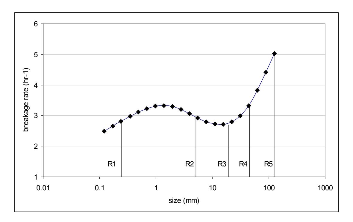
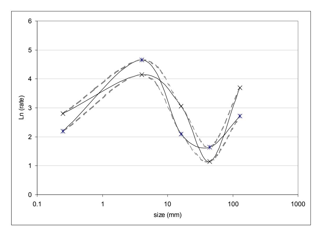
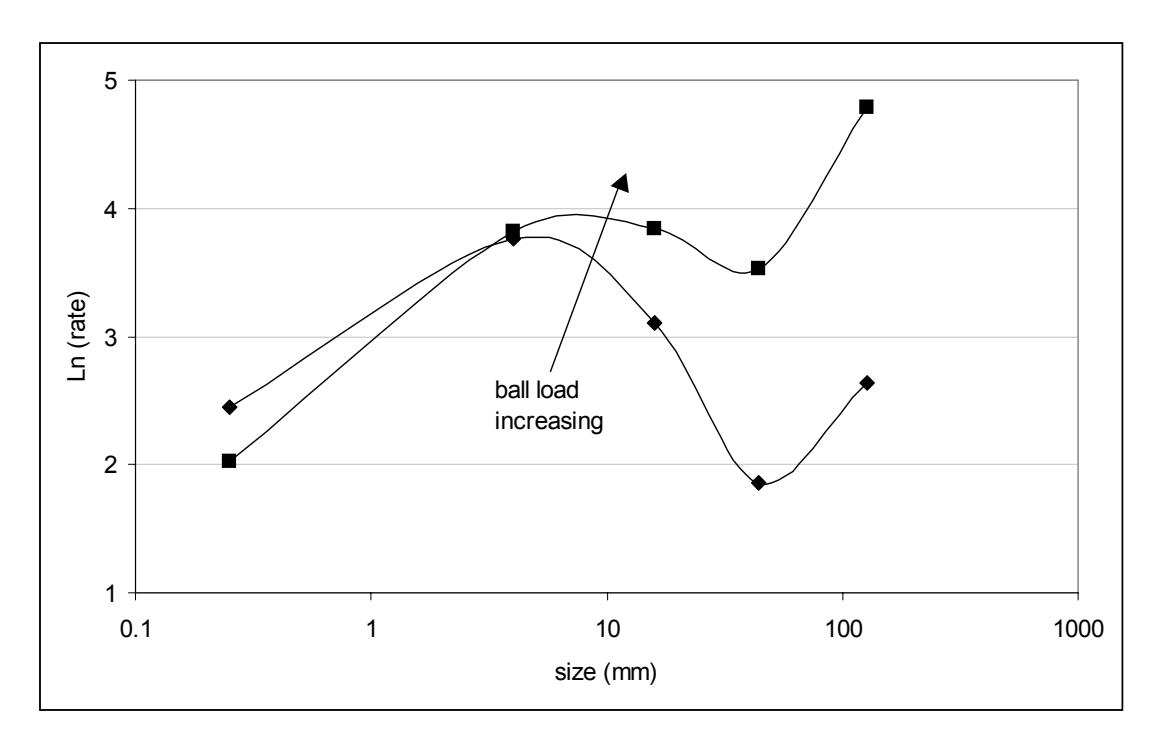
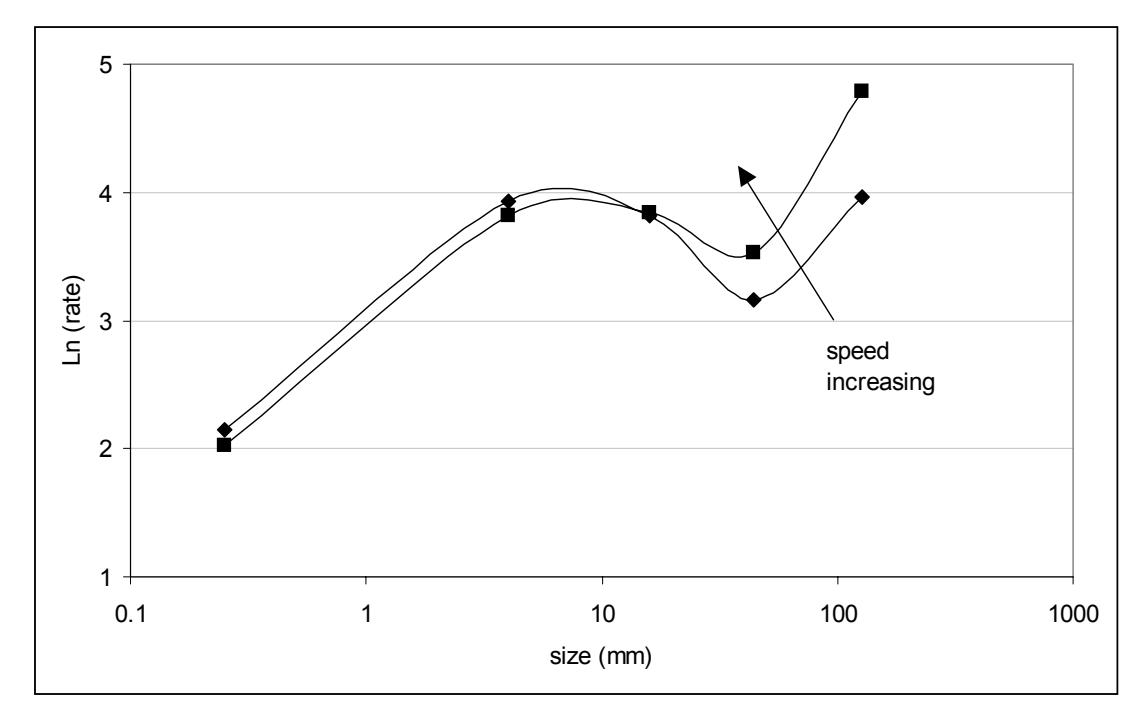
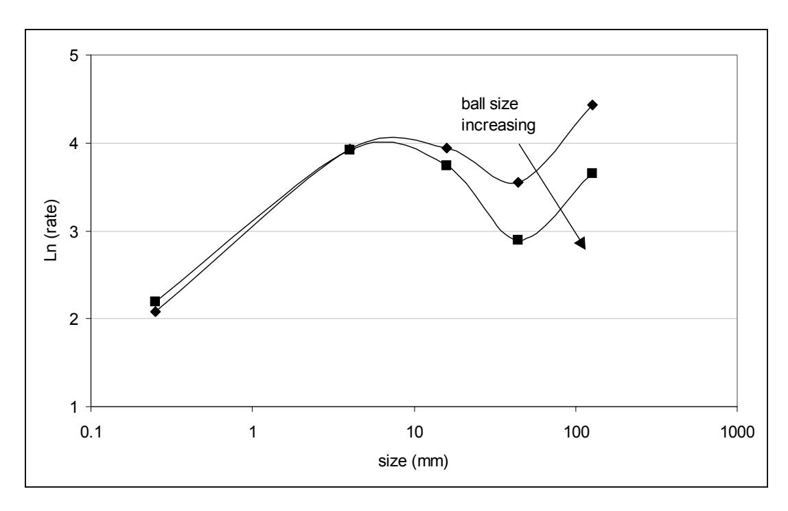
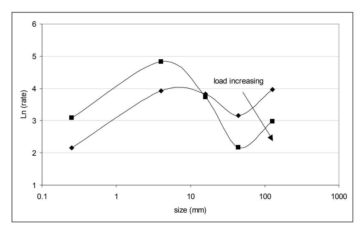
Although the general shape shown in Figure 3 appears to be maintained for a wide range of conditions it varies in a systematic manner with factors such as ball load (Morrell and Morrison, 1996) and total charge volume (Morrell et al, 2001). However, there is a major problem with determining what the exact variation is, which is related to the difficulty in obtaining load size distributions. From equation 1 it can be seen that without a load size distribution the breakage rate cannot be calculated directly. The data used to construct Figure 3 were obtained from an audit of a 7m SAG mill whose entire rock, slurry and ball load of 150 tonnes was removed separated and sized (Morrell, 1989). This task was extremely time consuming and costly and is not practicable for the frequencies necessary to obtain the required mill design and operational dependencies of the breakage rate distribution. However, it is possible using data fitting techniques to estimate the breakage rate distribution without a load size distribution. The feed, product and breakage distribution function must still be known, but in this case a non-linear fitting routine is used to simultaneously estimate both the breakage rate and load size distribution. This can be done by choosing the load size and breakage rate distribution that best predicts the observed product size distribution. The criterion of minimising the sum of the squared deviations between the observed and predicted sizings of the product stream is normally used for this purpose. The problem with this approach is that there is often a range of solutions that give very similar results in terms of the goodness of fit. This is illustrated in Figure 4, which shows 2 different breakage rate distribution that were fitted to a single a set of data in which the load sizing was not available. The breakage rate distributions gave almost identical fits to the product sizing. Together they define an envelope, within which the true distribution is expected to fall. The magnitude of envelopes such as these makes the experimental determination of trends in the breakage rate distribution difficult to define with precision.

Another solution to the problem is to use pilot mill data, as it is much easier to obtain load sizings. However, the question then arises as to whether the trends seen in pilot mill breakage rates are repeated in full scale mills. To help answer this question data from 11 different pilot scale tests were analysed and compared to the results obtained from the full scale mills that were subsequently built to treat the same ores. The results are given in Figure 5 and shown the average pilot scale distributions for the 11 pilot tests compared to the average from the 11 full scale mills. A distinct difference between the 2 distributions is seen. This is principally attributed to the influence of the rate of rotation (not diameter, which might be the first conclusion drawn from the data). The reason for attributing the differences to the rate of rotation (rpm) is that the energy calculation algorithm should have accounted for the influence of mill diameter via its relationship to breakage energy. As the breakage rate is related to breakage frequency (it has the same units) it is considered to be more likely that the differences are related to the frequency with which the mill rotates. For the same fraction of critical speed the rotational rate of a pilot mill is much higher than a full scale mill and hence it is believed that the higher rates at coarser sizes exhibited in Figure 5 are due to this. The obverse result at finer sizes is thought to be related to the much higher numbers of grinding media layers that are present in the bulk of the charge in full-scale mills. It is between these layers that much of the grinding of finer particles is thought to take place.

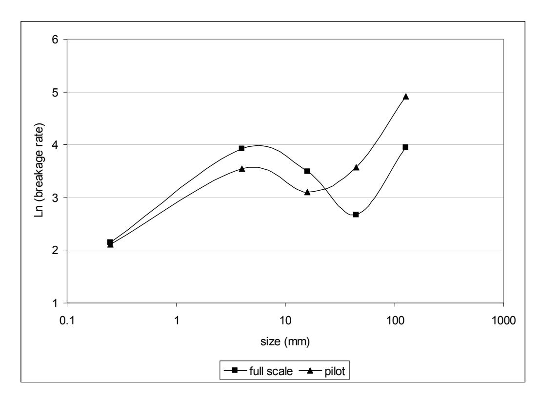
Given the effect of scale and the need to translate trends from the pilot scale to those at full scale it was decided to use the 11 data sets with their matching pilot and full scale conditions to develop the breakage rate relationships. This was done through a series of equations that related the rates R1-R5 to operational conditions (including rpm). This follows a similar approach to that originally developed by Mutambo (1993) and Morrell and Morrison (1996) in the JKMRC's so-called "variable rates model". Different equations were obtained to these earlier works, the general form being as follows:

$$ Ln(R_i) = k_{i1} + k_{i2}J_bD_b + k_{i3}\omega + k_{i4}(J_t) $$ (10)

where

Ri = breakage rate values for rates i = 1-5

Jb = % by volume of balls

Jt = % by volume of grinding media (ball plus rocks)

Db = make-up ball size

ω = mill rotational rate

ki1-i4 = constants for rates i = 1-5

The resultant equations gave a set of responses to changes in ball load, ball size, total load and speed which are illustrated in Figures 6-9 as well as matching the differences between pilot and full scale shown in Figure 5.

Power Draw

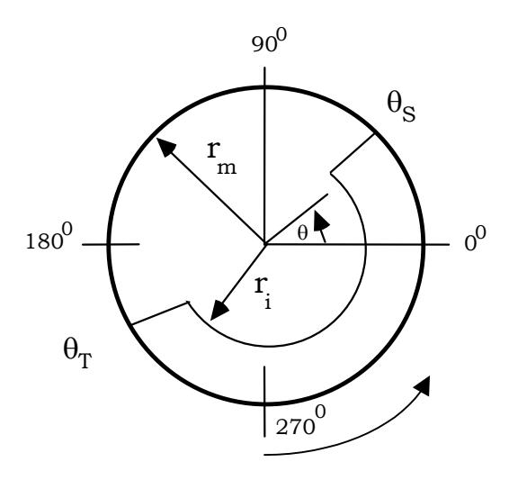
The size reduction part of the model predicts what the mass of rock and the quantity of slurry will be in the mill for a given feed rate. The power model uses this information to predict what the volume, density and position of the charge will be. The position of the grinding media portion of the charge is described using the conceptual view shown in Figure 10 (Morrell, 1996).

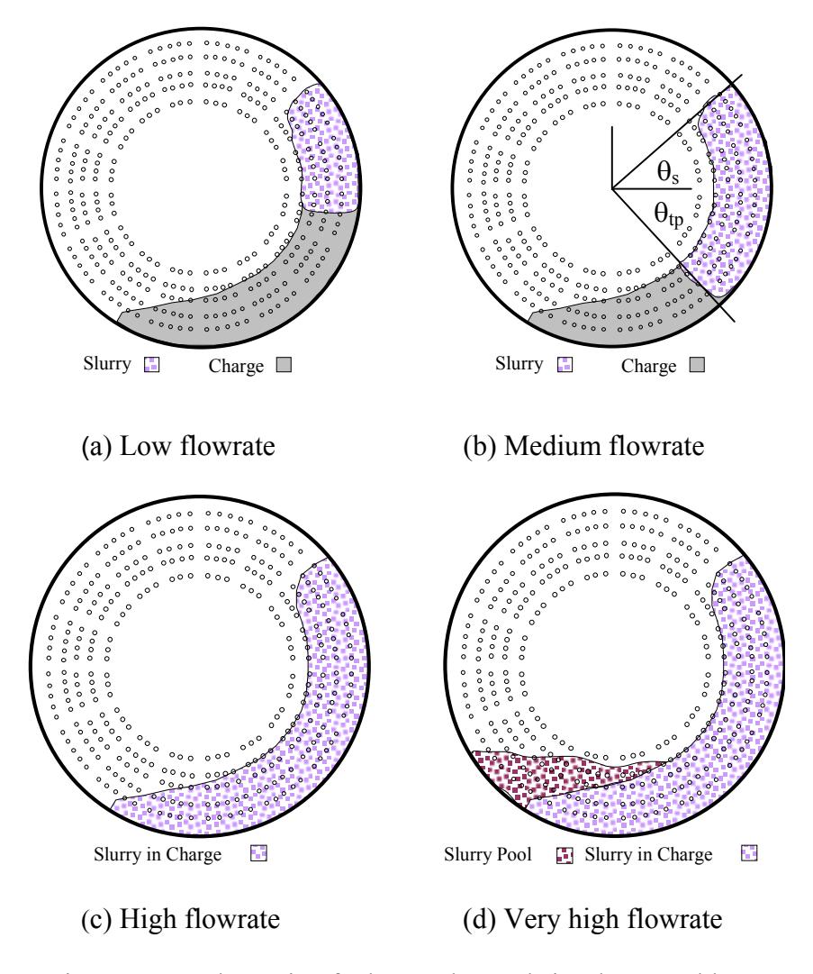
The slurry portion of the charge occupies the grinding media interstices. However, it is not uniformly dispersed but fills the interstices from the shoulder down towards the toe of the grinding media charge (Latchireddi and Morrell, 2003). This it does so in response to changes in the slurry flowrate. The toe of the slurry portion of the charge is therefore not necessarily coincident with that of the grinding media. This is illustrated schematically in Figure 11, which shows the movement of the slurry toe as flowrate increases. If the flowrate is high enough a slurry pool forms (Figure 11d) in which case the slurry toe effectively extends beyond the grinding media toe. This situation occurs in all overflow discharge ball mills and gives rise to the lower power draw which is usually seen in overflow ball mills compared to grate discharge units with the same size, ball charge and speed. It also causes the drop in power seen in AG/SAG mills that are fed at a rate that is too high for the grate/pulp lifters to handle (Morrell and Kojovic, 1996).

Using an energy balance approach, where power is taken to be the rate at which potential and kinetic energy is imparted to the charge, equation 11 was developed for the cylindrical section of the mill. Some mills have conical end-sections and, as they also draw power, have to be included if accurate predictions are to be obtained. Equation 12 was therefore developed and describes the power draw of a single conical end-section.

$$ P_{cylinder} = \int_{r_s}^{r_m} (V_r Lrg(\rho_c(\sin\theta_s - \sin\theta_t) + \rho_p(\sin\theta_s - \sin\theta_{tp}))dr $$ (11)

$$ P_{cone} = \int_{0}^{L_i} \int_{r_i}^{r_c} (V_r rg(\rho_c(\sin\theta_s - \sin\theta_t) + \rho_p(\sin\theta_s - \sin\theta_{tp})) dr dL_c $$ (12)

where,

Lc = length of cone-end, measured from the cylindrical section, at a radius of rc

Li = length of charge surface within cone ends

L = length of cylindrical section of the mill inside liners

P = power delivered to the charge (net power)

r = radial position

ri = radial position of charge inner surface

rm = radius of mill inside liners

rc = radius of cone-end at a distance Lc from the cylindrical section (m)

Vr = tangential velocity of a particle at radial distance r

θs = angular displacement of shoulder position at the mill shell

θt = angular displacement of the grinding media toe position at the mill shell

θtp = angular displacement of the slurry toe position at the mill shell (see Figure 11b

ρc = density of rock/ball charge (excluding pulp)

ρp = density of pulp phase

The variation in the angles (θs,θt), as well as the velocity variation with radial position (Vr), were modelled empirically from observations of the charge in a glass laboratory mill (Morrell, 1993).

Equations 11 and 12 describe the net power draw and do not include electrical and mechanical losses. To predict the total (gross) power draw these losses must be added to the net power. A further equation is therefore required which relates these losses to the mill's dimensions and speed. The no-load power equation proposed by Morrell (1996a) was used for this purpose.

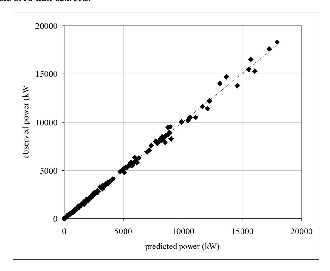
The resultant model should be applicable to all AG and SAG mills as well as ball mills. The accuracy of the model is demonstrated in Figure 12 using 140 ball, AG and SAG mill data sets.

MODEL VALIDATION

To test the validity of the model data from 21 different full scale AG/SAG mill circuits were used. The data comprised mill dimensions, grate design, mill speed, throughput, feed size distribution, product size distribution, power draw, ball load, ball size, normal operating load level and rock breakage characteristics (JK A and b values). The range in the major variables covered by the data sets is given below. ball load: 0-17% by volume

ball size: 100-150mm

total load: 20-40% by volume speed: 68-80% of critical

diameter: 1.7-12 m

length: 0.5-12 m aspect ratio (L/D): 0.33-1.85

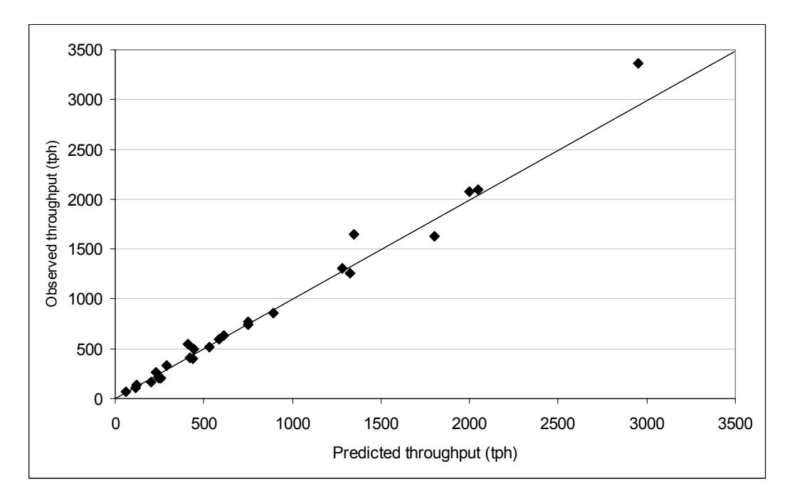
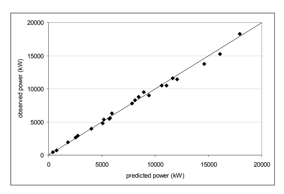
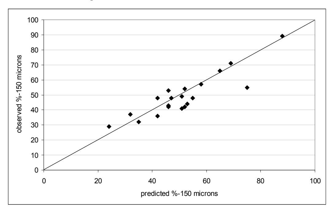
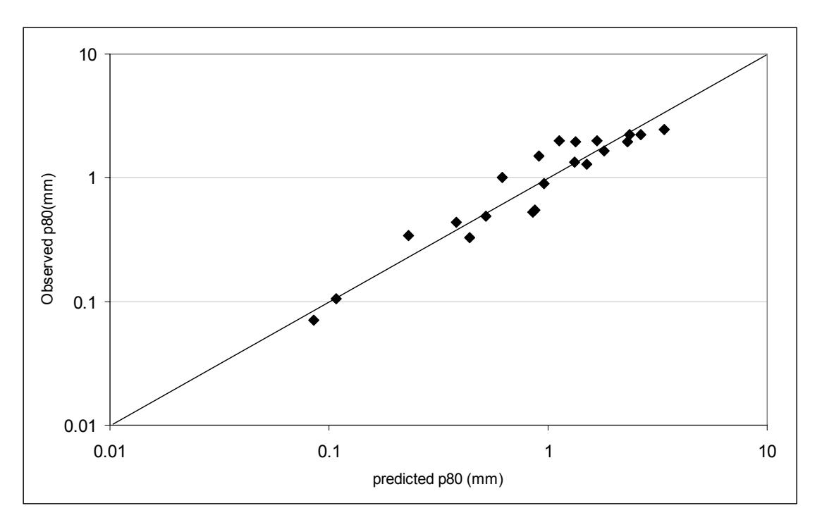
The simulations were run by first inputting the design and operational conditions as well as the JK A and b parameters. The breakage rate distribution was then predicted. Then, using the observed feed size distribution the throughput was increased until the observed total charge level was reached. The resultant power draw, throughput and product size distribution predictions of each circuit were then compared to those measured in the field. The results are given in Figures 13-16. The throughput and power draw were found to be predicted with a reasonable high degree of accuracy. The predicted product sizes followed the observed values well though more scatter in the data were apparent in comparison to the predicted throughput and power draw results.

CONCLUSIONS

A new AG/SAG mill model has been developed which incorporates some of the tried and proven elements of a number of previous models as well introducing a number of recent developments, particularly in the field of slurry transport. The model was refined using a suite of full-scale mill data that had complementary pilot-scale data. Validation of the resultant model was carried out using results from 21 full-scale mill circuits. It was shown that the model provided good predictive capability in terms of throughput and power draw as well as being able to follow product size trends well. The model should find application as a stand-alone design tool, to scale-up from pilot data and to optimise existing circuits.

REFERENCES

Ahlberg, J. H., Nilson, E.N. and Walsh J.L. 1967. The theory of spline functions and their applications. Academic Press, New York.

Austin,L.G., Menacho,J.M. and Pearcy, F., 1987.A General Model for Semiautogenous and Autogenous Milling, Proc. 20 th. Int. Symp. of Applications of Computers and Maths in Mineral Industries, Vol. 2 : Metallurgy,SAIMM: 107-126

Austin,L.G., Weymont, N.P., Barahona, C.A.,Suryanarayanan K.,1985.An Improved Simulation Model for Semi-Autogenous Grinding,SME-AIME, 85: 378 pp

Austin,L.G.,Weymont, N.P.,Prisbrey, K.A., and Hoover, M., 1976. Preliminary Results on the Modelling of Autogenous Grinding. 14 th Int. APCOM Conf., The Penn. State Univ.: 207-226

Barahona, C.A., 1984. Modelling and Simulation of Semi-Autogenous Grinding Systems. M.Sc. Thesis,The Penn. State University.

Epstein, B., 1947. The material description of certain breakage mechanisms leading to the logarithmic-normal distribution. J Franklin Inst, 244-471

Leung, K.,1987. An Energy Based Ore Specific Model for Autogenous Grinding Mills, Ph.D Thesis. University of Queensland, Australia.

Latchireddi, S R., 2002. Modelling the performance of grates and pulp lifters in autogenous and semi-autogenous mills. PhD thesis. University of Queensland. Australia.

Latchireddi, S R. and Morrell, S. 2003. Slurry Flow in Mills: Grate-only Discharge Mechanism. Minerals Engineering (In Press)

Morrell, S., 1989. Simulation of bauxite grinding in a semi-autogenous mill and DSM screen circuit. M.Eng thesis. University of Queensland. Australia

Morrell, S., 1993. The prediction of power draw in wet tumbling mills. PhD thesis. University of Queensland. Australia

Morrell, S. 1996. Power draw of wet tumbling mills and its relationship to charge dynamics - Part 1: a continuum approach to mathematical modelling of mill power draw. Trans Inst Min Metall, Section C Vol 105, C43-53.

Morrell, S. 1996. Power draw of wet tumbling mills and its relationship to charge dynamics - Part 2: an empirical approach to modelling of mill power draw. Trans Inst Min Metall, Section C, Vol 105, C54-62.

Morrell, S and Kojovic, T., 1996. The influence of slurry transport on the power draw of autogenous and semi-autogenous mills, Proc. Of 2nd Int. Conf. on Autogenous and Semi-autogenous Grinding Technology, Vancouver, Canada., pp.378-389.

Morrell, S. and Morrison, R.D. 1996. AG and SAG mill circuit selection and design by simulation, Proc SAG '96, Vancouver, Vol 2 pp769-790.

Morrell, S and Stephenson, I., 1996. Slurry discharge capacity of autogenous and semi- autogenous mills and the effect of grate design. Int. J. Miner. Process, 46(1-2) : 53.

Morrell, S., Valery, W., Banini, G. and Latchireddi, S., 2001. Developments in AG/SAG Mill Modelling. Proc. Int. Conf. Autogenous and Semi-autogenous Grinding Technology, vol 1V, pp.71-84.

Mutambo, J., 1993. Further Development of an Autogenous and Semi-autogenous Mill Model. M. Eng Sci. Thesis . University of Queensland. Australia

Napier-Munn, T.J., Morrell, S., Morrison, R.D. and Kojovic, T., 1996, Mineral Comminution Circuits Their Operation and Optimisation. JKMRC Monograph Series.

Narayanan, S. S. and Whiten, W. J., 1988. Determination of comminution charctersitics from single particle breakge tests and its application to ball mill scaleup. Trans Inst Min Metall, 97, C115-124.

Nordell, L. K., Potapov, V. and Herbst, J. A., 2001, Comminution Simulation Using Discrete Element Method (DEM) Approach – From Single particle Breakage to Full-Scale SAG Mill Operation. Proc SAG 2001, Vancouver, vol IV pp 235-251

Stanley, D.D., 1974,The Autogenous Mill- a Mathematical Model Derived from Pilot and Industrial Scale Experiment, Ph. D. Thesis (Unpublished),University of Queensland, Australia

Weymont, N.P.,1979. The Analysis and Simulation of Autogenous Grinding Systems. PhD Thesis ,The Penn. State Univ.

Whiten W. J. 1974. A matrix theory of comminution machines. Chem Eng Sci, 29, 588-599