



The content on this page was automatically generated from the PDF publication document and may contain errors or inaccuracies. Please refer to the original PDF for the most accurate information.
A Novel Approach to the Geometallurgical Modelling of the Collahuasi Grinding Circuit
O.M. Alruiz a , S. Morrell b , C.J. Suazoa , A. Naranjo a
a. Compañia Minera Doña Inés de Collahuasi SCM
b. SMCC Pty. Ltd..
Abstract
Compañía Minera Doña Inés de Collahuasi SCM (Collahuasi) initiated the development of a new geometallurgical model to characterize its Rosario deposit in terms of its comminution circuit capacity and flotation performance. The comminution component of the model is now complete and is described in detail.
The model uses a combination of simulation and power-based approaches to relate ore hardness and flotation feed size to grinding circuit throughput. Ore hardness values are provided by Collahuasi's block model which has been populated with ore characterisation data derived from Bond ball work index tests, JK drop-weight tests and SMC Tests® on diamond drill cores. The influences of planned and unplanned maintenance downtime are taken into account both in terms of frequency and duration.
The accuracy of the model is demonstrated using weekly production data taken from the period January-October 2008, indicating an overall accuracy of 4.9% and an R2 value of 0.95.
The model is now in successful routine use at the mine for planning purposes and is currently in the process of being further developed to incorporate the response of the flotation circuit.
Keywords : Girnding; Modelling; Simulation; Sulphides Ore
1. Introduction
As Walters and Kojovic (2006) stated "Geometallurgy is not new", though in recent years many mining companies have invested significantly in this area as they have increasingly realised that constructive integration of geology, mining and processing aspects into a socalled "Geometallurgical model" pays financial dividends through being able to maximise the throughput and efficiency of their treatment plants in both short and long-term time frames. The popularity of such modelling has been spurred on by advances in our understanding of how Autogenous (AG), Semi-autogenous (SAG) and ball mills behave, plus developments in ore characterisation techniques relevant to AG and SAG mills that can be obtained from small diameter drill core (Morrell, 2004).
In practice, from a comminution perspective, an effective Geometallurgical model should be able to accurately forecast the throughput of the grinding circuit from information provided by the mine plan on the nature and quantity of ores that are to be delivered to the processing plant. To do so there are at least five important requirements of the model. These are that:
- sufficient and relevant samples have been identified, extracted and tested to ensure the required definition and resolution on a block-by-block basis in the mine plan;
- appropriate breakage tests have been chosen to describe comminution properties of the different rock types (units) in the ore body;
- the model(s) chosen to describe the comminution equipment in the circuit respond realistically to changes in breakage properties as described using the chosen breakage tests;
- all of the above are integrated into an overall description of the on-line operational response of the grinding circuit that takes into account non-ore related influences and which can be easily integrated into the existing block model.
- the final model can convincingly demonstrate its accuracy through validation using real operational data.
Each of these aspects has been comprehensively tackled at Collahuasi in its development of a Geometallurgical model for its "Rosario" deposit and will be described in the ensuing sections.
2. Ore Body Description
2.1 Location
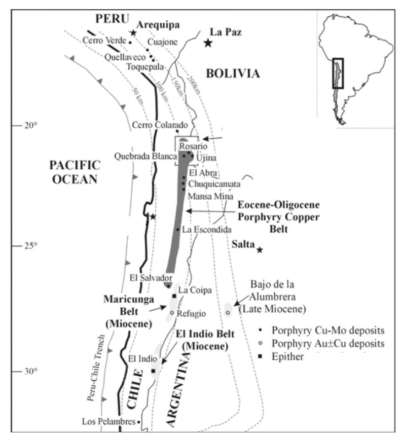
The Rosario mineral deposit is a copper and molybdenum porphyry with ore reserves of approximately 2.2 billion tonnes with an average copper grade of 0.82%. The Rosario pit is located 120 km southeast of the city of Iquique in the so-called Domeyko Cordillera at elevations ranging from 4,000 to 4,900 meters above sea level. As other large copper deposits in the North of Chile, this one is located in the northern end of the metallogenic strip of copper porphyries from the Eocene - Oligocene epochs, which includes Ujina, Quebrada Blanca, Chuquicamata and Escondida among other important deposits (see Figure 1).
2.2 Definition of Geometallurgical Units
The definition of the geometallurgical units was made in two stages, important components of which were based on previous work developed by the Xstrata Process Support Group, Canada (Fragomeni et al., 2005; Lotter et al., 2002). These stages involved firstly grouping the geometallurgical units on the basis of geological similarities and secondly determining their volumetric representivity in the material that was planned to be processed in the 5 year period 2008-2012 (the limit of the current modelling project).
The final result from this process was the development of six units that were considered to be representative of the deposit, these being labelled UGM 1-6 (UGM coming from the Spanish "Unidad GeoMetalurgica"). The proportions of each which are due to be mined over the period 2008-2012 are given in Table 1.
| UGM | Ore | UGM Proportion (%) |
|---|---|---|
| 1 | Primary | 18 |
| 2 | Primary | 26 |
| 3 | Primary | 19 |
| 4 | Primary | 25 |
| 5 | Secondary | 7 |
| 6 | Secondary | 5 |
3. Sample Selection and Laboratory Treatment
A total of 3000m of diamond drill core was extracted for the purposes of metallurgical testwork for this project and included 1500m of PQ (nominal 85mm) and 1500m of HQ (nominal 65mm) cores. The cores were chosen to ensure good spatial representivity and to ensure that the selected intervals also represented the average grades as well as the relative abundance of the various geometallurgical units.
The comminution tests selected to characterise the different units were the JK Tech dropweight test (Napier Munn et al, 1996) the SMC Test® (Morrell, 2004) and the Bond ball work index test (Bond, 1961). Composites using the PQ core were made up to represent each of the six UGM classes and JK drop-weight and Bond ball work index tests were carried out on these. Over 100 samples were also subjected to SMC Tests® and Bond tests using the HQ cores to provide variability details.
4. Experimental Results from Laboratory Tests
4.1. Grinding results on average composites
Table 2 shows a summary of the main laboratory test results obtained from the composite sample testwork program.
| UGM | parameter | UGM1 | UGM2 | UGM3 | UGM4 | UGM5 | UGM6 |
|---|---|---|---|---|---|---|---|
| average | |||||||
| A | 59.1 | 61.7 | 63.6 | 49.5 | 58.9 | 61.6 | |
| JK Drop-weight | b | 0.9 | 0.6 | 0.8 | 1.2 | 0.8 | 1.0 |
| testing parameters | ta | 0.80 | 0.73 | 0.64 | 0.78 | 0.56 | 0.95 |
| A*b | 52.6 | 37.0 | 52.8 | 59.4 | 49.5 | 58.5 | |
| Standard Bond Ball | |||||||
| Mill Wi | KWh/t | 10.5 | 12.5 | 10.5 | 11.4 | 10.7 | 9.9 |
| Specific Gravity | SG | 2.61 | 2.90 | 2.58 | 2.57 | 2.66 | 2.69 |
From Table 2, it can be observed that UGM 2 is relatively hard compared to the other units (note that with the JK drop-weight parameters a harder ore has a lower value of the parameter A*b). This unit represents 26% of the total that will be processed within the period 2008-2012. The Bond indices tend to be relatively soft for ball mill grinding.
However, as in the case of the JK drop weight tests, UGM 2 is indicated to be the hardest unit.
4.2. SMC Test® and Bond Work Index Variability Tests
Tables 3 and 4 show the SMC Test® and Bond ball work index test variability results respectively for each UGM. From an A*b perspective it can be seen that the UGM 4 and 5 units have a relatively high degree of variability. UGM 4 has similarly high variability in terms of the Bond ball work index.
| Variability Samples | ||||||
|---|---|---|---|---|---|---|
| Average on | Number of | Simple | Standard | |||
| SMC, A x b | composite sample | Samples | average | Deviation | Min | Max |
| UGM1 | 52.6 | 17 | 43.8 | 6.6 | 36.3 | 59.6 |
| UGM2 | 37.0 | 21 | 32.2 | 7.2 | 24.0 | 52.6 |
| UGM3 | 52.8 | 14 | 50.4 | 10.5 | 36.6 | 71.4 |
| UGM4 | 59.4 | 19 | 50.5 | 29.0 | 28.5 | 131.5 |
| UGM5 | 49.5 | 37 | 65.5 | 36.9 | 35.4 | 212.5 |
| UGM6 | 58.5 | 13 | 62.6 | 15.6 | 42.0 | 86.9 |
Table 4 shows the Bond test results on variability samples per UGM.
| Variability Samples | ||||||
|---|---|---|---|---|---|---|
| Bond Work Index, Wi, | Average on | Number of | Sample | Standard | ||
| kWh/t | composite sample | Samples | average | Deviation | Min | Max |
| UGM1 | 11.5 | 14 | 12.5 | 1.8 | 9.6 | 14.9 |
| UGM2 | 13.7 | 13 | 13.8 | 1.5 | 11.6 | 16.5 |
| UGM3 | 11.5 | 9 | 11.3 | 1.0 | 10.2 | 13.3 |
| UGM4 | 12.6 | 13 | 12.2 | 2.3 | 8.2 | 15.3 |
| UGM5 | 11.8 | 4 | 12.2 | 1.2 | 10.8 | 13.5 |
| UGM6 | 10.9 | 11 | 11.1 | 0.8 | 10.1 | 12.6 |
5. Collahuasi Grinding Circuit Description
The Concentrator operating facilities starts with the primary crusher at the Rosario pit. Crushed ore is transported by overland conveyor to the coarse ore stockpile in front of the three grinding SAG mills. The initial circuit included two grinding lines and achieved full production in October 1998. A third grinding line was installed during a subsequent expansion, with full production achieved in April 2004. The first two identical grinding lines (Lines 1 and 2) consist of one 32 x 13.5ft (8,000 kW installed power) SAG, in series with one 22 x 36ft (8,000 kW) ball mill each one. The third grinding line (Line 3) consists of one 40 x 22ft (21,000 kW) SAG mill working with two 26 x 38ft (15,500 kW each) ball mills, the SAG mill currently being the largest of its kind in the world. SAG mill trommel oversize product (pebbles) is sent to the pebble crushing plant, consisting of two pebble crushers in parallel. Crushed pebbles are returned to the coarse ore stockpile. Ball mills work in a reverse classification circuit, wherein the hydrocyclone underflow feeds into the ball mills and the hydrocyclone overflow is sent to the flotation circuit.
The current daily average throughput of Collahuasi´s grinding circuit is 130.000 tons per day with an average product size (P80) of approximately 200 microns.
6. Comminution Circuit Modelling
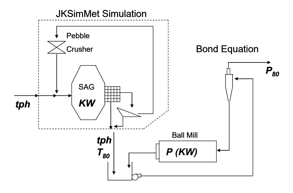
To represent the performance of the SAG mill circuit it was decided to use JK Tech's comminution simulator – JKSimMet, whilst the power-based equations of Bond were chosen for the ball mill circuit (Bond, 1961). The so-called variable rates model (Morrell and Morisson, 1996) was used to simulate SAG mill performance, model parameters being fitted using data from surveys of the circuit undertaken in 2006.
JKSimMet is proprietary software and could not be easily integrated with the Collahuasi block model software. To overcome this problem a series of simulations of the SAG mill circuit were run in which the throughput was incrementally varied and the power draw and SAG mill circuit product size (so-called transfer size P80 or T80 for short) recorded. Operating conditions for the SAG mill such as ball load, speed and % solids were kept constant as they are during normal plant operation. This was done up to throughputs that resulted either in the predicted power draw reaching 90% of installed power or the combined ball and rock load reaching 30%, these being practical limits dictated by actual plant operation. This procedure was carried out for each of the UGM units using the JKTech A and b values as presented in section 4. For each UGM each throughput and associated transfer size was then put into equation 1.
Where, P is the ball mill circuit power draw, Wi is the Bond laboratory work index for the selected UGM, tph is the SAG circuit throughput, P80 is the ball mill circuit final grind P80 and T80 is the SAG mil circuit transfer size for the selected UGM and at the throughput indicated by "tph". Rearranging equation 1 gives equation 2 from which the ball mill circuit final grind (P80) can be estimated:
A schematic illustrating this process is given in Figure 2.
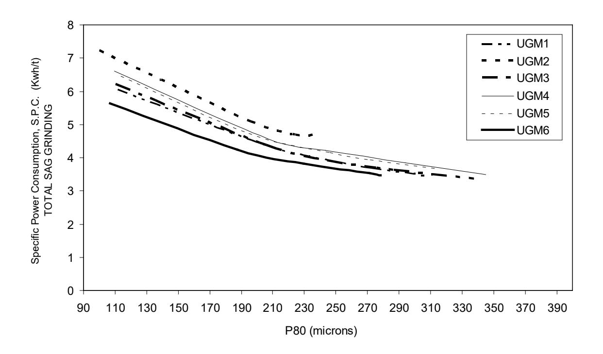
Having related SAG mill throughput to SAG mill power and the ball mill circuit P80, the data were then reduced to a series of curves representing the relationship between the SAG mill specific power consumption (S.P.C), which is the SAG mill power draw divided by throughput, and the ball mill P80 for each UGM. Figure 3 shows the six resultant plots. The terminal points in each plot (at coarser P80 values) are associated with reaching the SAG mill limit of 90% of installed power or 30% load. From Figure 3 it can be observed that when the P80 increases the predicted SAG specific power consumption (kWh/t) decreases. This phenomenon is driven by the fact that in SAG mills, particularly those with high ball loads, the power draw of the mill is dominated by the ball charge. When the SAG mill is being underfed and hence the throughput is relatively low the kWh/t is relatively high. As throughput is increased the rock load builds in the mill though its influence on the power draw is relatively small and disproportionate to the throughput increase. As a result the SAG mill power goes up by a relatively small amount compared with the throughput increase and hence the SAG mill kWh/t drops. In the ball mill circuit, however, the higher throughput is translated into a coarser P80. Hence, as the SAG mill kWh/t decreases the ball mill circuit P80 increases. It should be noted that this response is usual for circuits that are mostly ball mill capacity limited. Where the circuit is SAG mill capacity limited and the ball mill has excess capacity, operational practice is often to target a specific flotation feed size and to keep it at this value regardless of the SAG mill throughput and kWh/t. Collahuasi tends to be ball mill capacity limited and hence is operated in a way similar to that implied by equation 2.
A simple power model (Eq 3) was used to fit the S.P.C. curves shown in Figure 3.
The parameters J and K depend on the metallurgical unit and the grinding line (1-2 and 3). Table 5 summarizes the values for these parameters per grinding line. It is noticeable from the data in Table 5 that in general there is a systematic difference in the parameters between line 3 and lines 1-2. This is caused mainly by the differences in the relative amounts of ball mill power to SAG mill power, line 3 having more ball mill power in relation to SAG mill power than in lines 1 and 2. The different aspect ratios of the SAG mills will also have an influence as the higher aspect ratio of the line 3 mill is expected to produce a coarser transfer size and a lower specific energy than those in lines 2 and 3 (Morrell, 2007).
Equation 3 can now be used to estimate the circuit throughput for a given UGM by selecting the appropriate J and K values and choosing a target P80 for the ball mill circuit. This generates a S.P.C. value for the SAG mill. If the automatic SAG mill control is then set to a particular power draw then that power draw divided by the S.P.C. value should be the instantaneous throughput achieved by the grinding circuit. Blends of UGM units being fed to the mill are handled by producing a weighted average S.P.C. based on relative tonnage in the blend.
| Grinding line 3 | |||||
|---|---|---|---|---|---|
| J | K | ||||
|
UGM
1 |
79.82 | -0.57 | |||
|
UGM
2 |
65.84 | -0.51 | |||
|
UGM
3 |
82.20 | -0.58 | |||
|
UGM
4 |
82.54 | -0.56 | |||
|
UGM
5 |
89.61 | -0.58 | |||
|
UGM
6 |
58.79 | -0.53 | |||
|
Grinding line 1 -
2 |
|||||
|
UGM
1 |
86.67 | -0.53 | |||
|
UGM
2 |
87.84 | -0.50 | |||
|
UGM
3 |
77.92 | -0.52 | |||
|
UGM
4 |
94.83 | -0.54 | |||
|
UGM
5 |
101.79 | -0.55 |
|---|---|---|
|
UGM
6 |
67.06 | -0.49 |
7. Production Model
The S.P.C. versus P80 relationship of equation 3 is used to predict the instantaneous throughput of the circuit. In practice, however, throughput cannot be maintained at the predicted levels all of the time due to occasional interruptions or disruptions, usually as a result of maintenance-related shutdowns. These have both a direct and an indirect impact on production. The direct impact is the shutdown of the equipment that causes total or partial reduction in throughput whilst repairs are made. Additionally, throughput is limited during ramp-up after repairs are finished and in some cases also a ramp-down as the plant is made ready just prior to a maintenance shutdown. In these cases the plant is not at full capacity for several hours and this causes reductions in throughput that are not related to ore type. The ramp-up and ramp-down delays tend to be fixed durations (see later) and therefore the net effect is that not only does the duration of the shutdown have an impact on productivity but also the frequency with which they occur. Hence one long shut down will incur only one penalty of a ramp-up and ramp-down delay. Several shut downs with the same duration as the long one will incur several ramp-up and ramp-down delays, therefore causing a greater throughput loss.
To incorporate all of these influences the Production Model shown as Eq. (4) was developed as follows:
(4)
Where:
- Ton \( (P_{80}) \) : Is the total treatment capacity of the grinding circuit for a certain \( P_{80} \) within a period of time of H hours in total.
- \( T_{LI} \) : Is the average instantaneous throughput of grinding line 1 for a given target \( P_{80} \) . \( T_{LI} \) is obtained dividing the average specific power consumption by the SAG power draw. The average specific power consumption is the weighted average of the specific power consumption associated to each UGM (from Eq. (3)) by the proportions in which the units are fed in a period of time.
That is:
$$ S.P.C_{L1} = \sum_{i=1}^{6} S.P.C_{I1}^{UGMi}(P_{80}) \times f_{i} $$ (5)
Where \( f_i \) are the proportions of each UGM within the period of time, then:
Finally, the average throughput is calculated from Eq. (7) as follows:
\( S.P.C_{L1}^{UGMi}(P_{80}) \) is the specific power consumption of the SAG line 1 at a certain \( P_{80} \) when 100% of the UGMi is processed. The sub index "i" denotes the number of the unit, i.e., it takes values from 1 to 6.
• \( T_{L2} \) , \( T_{L3} \) are the same as \( T_{L1} \) , i.e., correspond to the instantaneous throughputs of grinding lines 2 and 3 for a certain \( P_{80} \) .
- H : Total of hours contained within the period of time, without deducting stops of any kind.
- Hml1, Hml2, Hml : Total of programmed maintenance hours at the grinding lines 1, 2 and 3, respectively.
- Hfl1, Hfl2, Hfl3 : Total of un-programmed maintenance hours at the grinding lines 1, 2 and 3, respectively. Historical information can be used as an estimator of this parameter.
- Nl1, Nl2, Nl3 : Number of shut downs within the analysis period of grinding lines 1, 2 and 3, respectively.
- Ht : Hours or transient period that a grinding line takes to achieve the stationary condition (full capacity). Statistically, 12 hours were observed in Collahuasi as transient periods. Assuming a uniform ramp-up for treatment increase, it was estimated a total of 6 hours of treatment loss for each stop in a grinding line.
- PTtchp : Treatment capacity losses caused by the pebbles crushing systems shut downs.
- Hmchp : Programmed maintenance hours at the pebbles crushing system.
- Hfchp : Un-programmed shut downs at the pebbles crushing system.
8. Validation
From January to October 2008 weekly data were collated from the production records. Information included throughput, SAG mill power draw, both the programmed and un programmed shutdown hours per grinding line, plus the ball mill circuit \( P_{80} \) per grinding line fed to the flotation circuit.
The proportions of each unit fed to the plant were obtained from the mining planning report for the period. In the case of Collahuasi, the shortest period that the model is expected to be accurate over is a week. The reason for this is the two stockpiles between the open pit and the SAG mills, which makes it difficult to know the exact proportions of each unit fed to the plant on a daily basis.
Using this information plus the "S.P.C. versus \( P_{80} \) " curves associated with each metallurgical unit for each grinding line, the average instantaneous throughput of each line was predicted, as follows:
In Equation (8), \( T_{Lj} \) is the average throughput of the grinding line "j" for a certain \( P_{80} \) . The average specific power consumption was estimated from Eq. (2), considering the proportions " \( f_i \) " of each unit within the period of analysis.
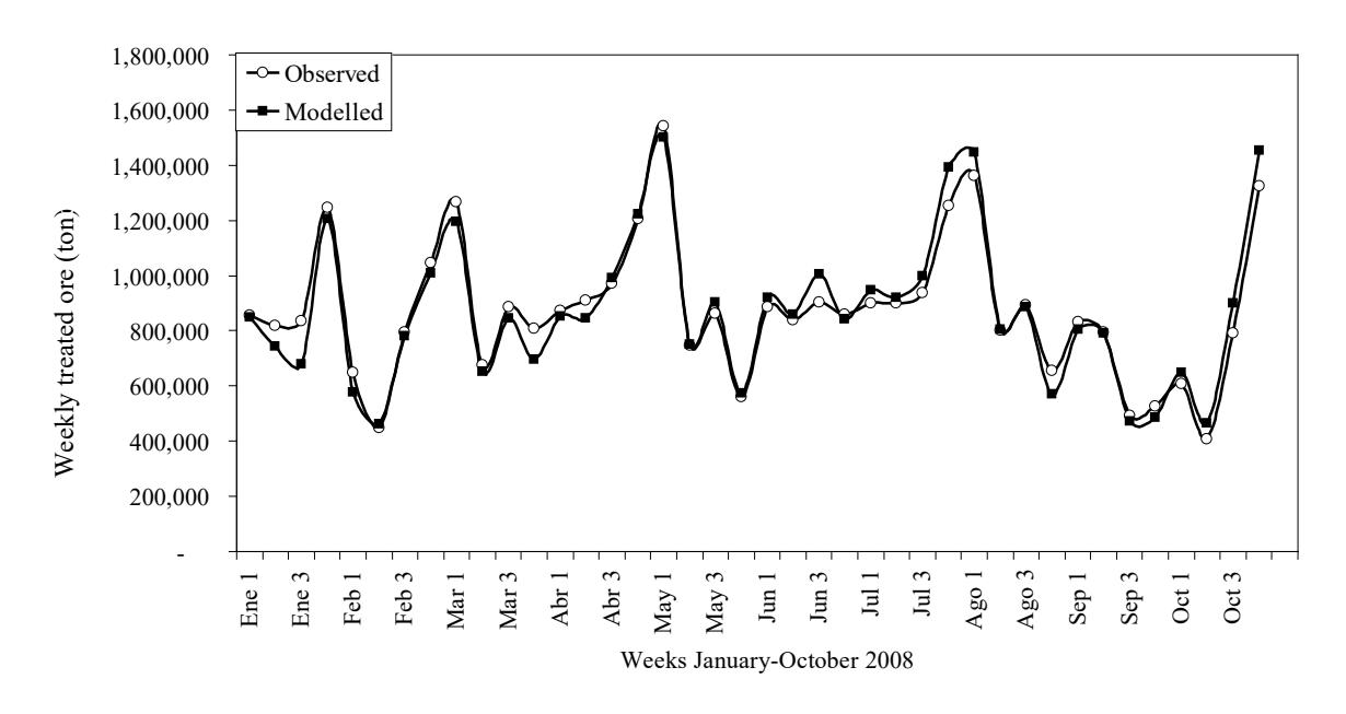
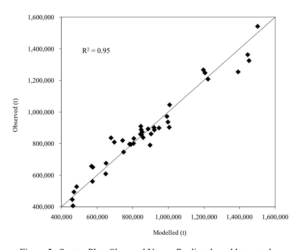
Subsequently Eq. (4) was used in order to estimate the total treated ore per week during 2008. Figure 4 shows the predictive capacity of the model for the period in question. As can be seen, the production model was able to satisfactorily predict the observed processed tonnages. Figure 5 shows the actual values versus the predicted average weekly throughput with an associated R2 value of 0.95. The calculated overall percentage error of the model was 4.9%.
9. Application of Collahuasi Treatment Model to Mine Planning
The production model is now programmed in such a way that planning engineers at Collahuasi are able to estimate the grinding circuits' treatment capacity for each mining plan that may be created. One advantage of this approach is that it allows the planning engineers to maximise treatment capacities on the basis of appropriate blending of UGM units and also on the basis of the concentrator's maintenance program. Another advantage of this approach is that it also allows the use of the P80 as an input for flotation circuit modelling. This latter model is currently under development but will ultimately be integrated with the grinding model. This will enable planning engineers to optimise copper production and hence maximise profit by appropriate selection of UGM unit mixtures and planned maintenance programs.
An example of application is presented in Figure 6. This shows the concentrator's treatment capacity in tonnes per day estimated for several periods at a certain P80. The proportion of each metallurgical unit fed to the plant is showed for each analyzed period.
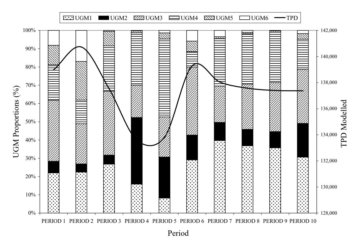
As can be seen from Figure 6, there are two periods where the expected throughputs are lower in comparison to the others (Periods 4 and 5). In those periods there is a high composition of UGM2 and UGM4, which are the hardest ores (see Figure 3).
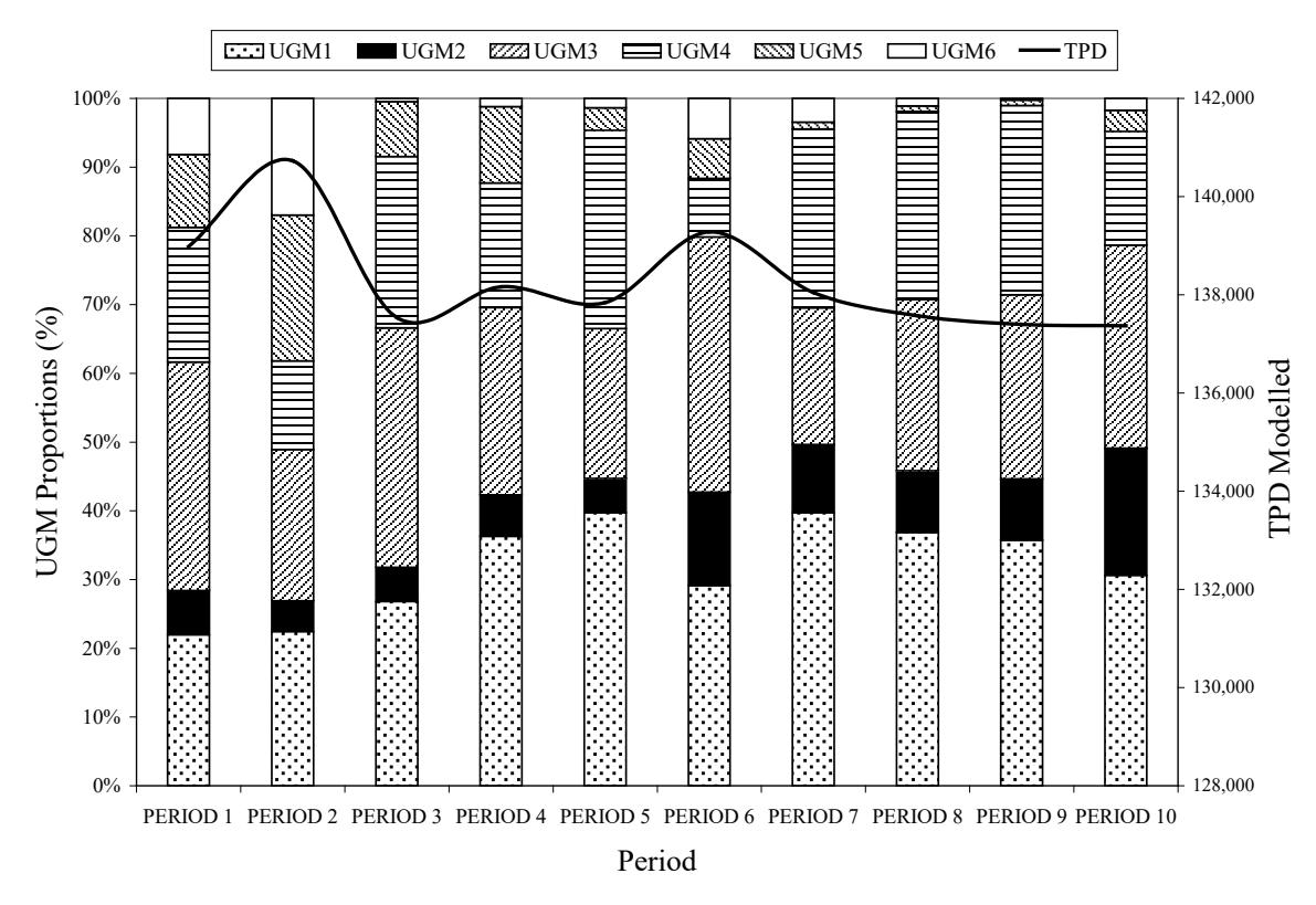
Figure 7 shows again the predicted throughput presented in Figure 6, but this time, the proportions of UGM2 and UGM4 in the periods 4 and 5 were diminished, increasing the amount of the other geometallurgical units. As can be seen from Figure 7, the expected throughput is smoothed and should lead to a much more stable circuit performance.
10. The effect of the un-programmed shutdown hours on treatment capacity
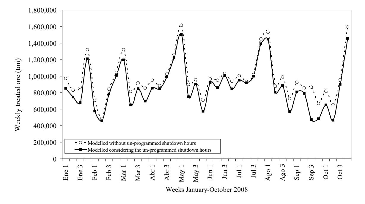
As mentioned in the previous section, one application of Eq. (4) is that planning engineers can modify the mining sequence of metallurgical units, i.e., adjust the proportions of UGMs planned to be fed into the plant, in order to ensure a certain level of throughput. A further novel application of Eq. (4) is that it allows the quantification of the impact of unprogrammed shutdown hours on plant throughput. In the case of Collahuasi unprogrammed shutdown hours are among the main reasons of low availabilities during certain periods. For example, Table 6 summarizes the Collahuasi observed availabilities obtained from the programmed and un-programmed shutdown hours within the period January to October 2008. When all the un-programmed shutdown hours are removed (Hfl1 = Hfl2 = Hfl3 = 0), the availabilities will improve resulting in an increase in the predicted throughput. Figure 8 illustrates this by comparing both the predicted throughput presented in Figure 4 and the predicted throughput when all the un-programmed shutdown hours are removed. The result was that if maintenance practices could be improved and the un-
programmed shutdowns reduced, the weekly throughput could have increased by 101,000 extra tons per week, i.e. about by 10%
|
Observed Values within the period
January-October 2008 Standard |
||||
|---|---|---|---|---|
| Grinding Line | Average | Deviation | Min | Max |
| Line 1 | 88.9 | 13.3 | 35.1 | 99.6 |
| Line 2 | 87.8 | 15.5 | 34.0 | 99.8 |
| Line 3 | 81.5 | 23.3 | 0.0 | 99.3 |
| Pebble Crusher | 81.2 | 13.0 | 49.1 | 100 |
14. Conclusions
The aim of developing a robust and accurate production forecasting model for the grinding circuit at Collahuasi has been satisfactorily achieved through the use of a combination of simulation and power-based modelling. This resulted in a model with an overall percentage error of 4.9% as judged by analyses using production data from the period Jan – Oct 2008.
It is believed that the accuracy of the model was due to:
- identification and selection of sufficient and relevant samples for characterisation purposes,
- use of appropriate breakage tests for characteristion,
- development of a robust model for describing comminution circuit performance,
- incorporation of non-ore related operational influences into the final throughput forecast model.
The model allows planning engineers to maximise grinding circuit treatment capacities on the basis of appropriate blending of UGM units and also on the basis of the concentrator's maintenance program.
Ultimately the model will be extended to incorporate the flotation circuit's response and hence enable optimisation to be done on the basis of metal recovery and hence profit.
15.Acknowledgements
The authors would like to thank Compañía Minera Doña Inés de Collahuasi for the support and the opportunity to develop this article.
16. References
Bond, F.C., 1961, Crushing and Grinding Calculation Part 1. British Chemical Engineering, 6(6), 378-385.
Fragomeni, D., Boyd, L.J., Charland, A., Kormos, L.J., Lotter, N.O. and Potts, G., 2005, The use of End-Members for grind-recovery modelling, tonnage prediction and flowsheet development at Raglan, In Canadian Mineral Processor , Ottawa, pp. 75-98
Lotter, N.O., Whittaker, P.J., Kormos, L.J., Stickling, J.S. and Wilkie, G.J., The development of process mineralogy at Falconbridge Limited, and application to the Raglan Mill. CIM Bulletin, 2002, 95(1066), 85-92.
Morrell, S., 2004. Predicting the specific energy of autogenous and semi-autogenous mills from small diameter drill core samples. Miner. Eng. (17/3), 447–451.
Morrell, S., 2007. The Effect of Aspect Ratio on the Grinding Efficiency of Open and Closed Circuit AG/SAG Mills. Proc. Ninth Mill Operators Conf., AusIMM, pp121–124
Morrell, S. and Morrison, R.D. 1996. AG and SAG mill circuit selection and design by simulation, Proc SAG '96, Vancouver, Vol 2 pp769-790.
Napier-Munn, T.J., Morrell, S., Morrison, R.D., Kojovic, T., 1996. Mineral Comminution Circuits: Their Operation and Optimization, JKMRC Monograph Series in Mining and Mineral Processing, vol. 2, University of Queensland, Brisbane, 413 p
Walters, S. and Kojovic, T. 2006. Geometallurgical mapping and Mine Modelling (GeM111) The way of the Future, Proc SAG '2006, Vancouver, Vol IV pp 411-425.