



The content on this page was automatically generated from the PDF publication document and may contain errors or inaccuracies. Please refer to the original PDF for the most accurate information.
AG AND SAG MILL CIRCUIT SELECTION AND DESIGN BY SIMULATION
Dr. S Morrell' and Dr. R D Morrison2 1- Manager - Comminution Research, 2- Manager, JKTech Julius Kruttschnitt Mineral Research Centre Isles Road, Indooroopilly, Brisbane, Australia
SUMMARY
The JKMRC AGISAG model typically requires a full scale plant or pilot mill survey combined with ore breakage testing to generate a set of grinding rates. However recent research using a large data base of pilot and full scale milling tests has lead to the development of a correlation between model grinding rates and mill operating conditions. A further correlation between mill feed sizing and ore breakage characteristics has also been developed. These two correlations now allow mill performance to be predicted for a wide range of mill sizes and operating conditions. Hence the model can be used to evaluate optimisation strategies in existing plants and to investigate (and compare) grinding circuit configurations at the pre-feasibility stage thus reducing the cost of pilot testing. A comparison of this design method vs actual measured performance including power is provided for a range of AGISAG mills and product sizes. The model is also used to describe in detail the effects of changing operating conditions.
Using these correlations the effects of changing operating conditions are considered in detail.
INTRODUCTION
Pilot-scale testwork based on a 6' x 2' mill is arguably still the most reliable method for predicting full scale autogenous (AG) and semi-autogenous (SAG) grinding mill behaviour when treating a given ore. However, the cost of a detailed pilot-mill programme both in terms of providing sufficient sample material as well as the hire of the plant can be prohibitive. Deposits with highly variable ore types are a particular problem as pilot testing of the different ore types greatly escalates the cost of the testwork programme.
The use of mathematical modelling and simulation based on laboratory ore characterisation can help reduce the cost of the pilot test programme. This can be achieved by both narrowing the choice of the most likely successful processing routes at the prefeasibility stage and providing realistic pilot plant throughput targets, as well as augmenting a pilot test programme on a bulk sample with a number of simulations based on satellite drill core samples. In cases where pilot-scale testwork is not possible, simulations referenced against a large industrial data base significantly reduces the risk of not piloting. The added advantages of the simulation route are in its versatility, its ability to simulate the entire comminution circuit and the ease with which combinations of circuit designs, operating conditions and ore types can be evaluated on a throughput, power utilisation and product size basis.
For 25 years the Julius Kruttschnitt Mineral Research Centre (JKMRC) has been conducting applied research on AGISAG milling. During this time it has collected a large volume of data from pilot and full size AGISAG mill grinding circuits as well as developing a number of ore characterisation tests with which to develop and validate its mathematical models. This paper describes some of the developments in the AGISAG model together with some examples of its use, with particular reference to the design of greenfield circuits.
MODEL STRUCTURE
In its original form the JKMRC AGISAG mill model utilises the concept that breakage within a mill is dependent upon specific breakage energy. This in turn is related to the mill dimension and a grinding medium size which is a characteristic of the ball charge (if any) and rock charge (Leung et al 1987).
The relationship between specific breakage energy and the progeny size distribution is provided by laboratory impact and tumbling tests which are carried out on the ore(s) in question. These generate breakage parameters which relate to the high energy (impact) and low energy (abrasion) size reduction processes which are believed to take place in AGISAG mills.
Transport of slurry through the mill is described by a function which relates the hold-up of slurry, grate design, grate open area and mill speed to the volumetric discharge rate through the grate (Morrell and Stephenson, 1996):
$$ J_p = kQ^{0.5}\gamma^{-1.25}A^{-0.5}\phi^{0.67}D^{10.25} $$ where
J, = fractional slurry hold-up
D = mill diameter (m)
y = mean relative radial position of the grate apertures
where
ai = open area of all holes at a radial position ri
r,= radius of mill inside the liners.
A = total area of the grate apertures (m2)
Q, = fraction of critical speed
Q = volumetric flowrate out of the mill (m3lhr)
Classification by the grate is related to the effective grate aperture by a simplified classification function. For illustrative purposes a conceptual view of the model is shown in Figure 1.
One of the limitations of the original model, particularly from a design viewpoint is that it contains a fixed breakage rate distribution, which must be back-calculated from existing plant data. However, it is clear from the many industrial and pilot data that have been examined that the breakage rate distribution varies considerably with factors such as ball load, mill speed and feed size (Morrell & Morrison, 1989; Morrell et al, 1995).
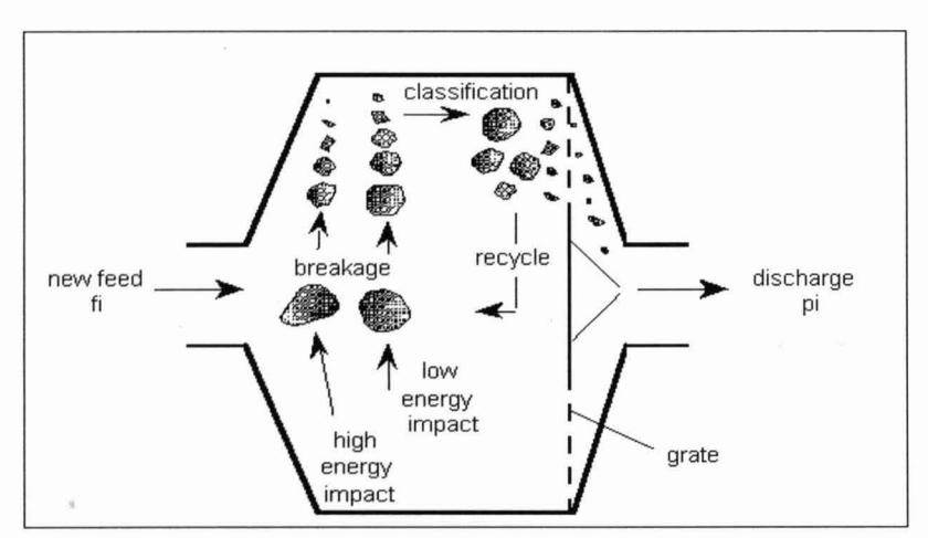
What is therefore needed is a relationship between operating conditions and the breakage rate distribution.
Breakage Rate Distribution
To determine what the relationship was between operating conditions and the breakage rate distribution systematic changes in the breakage rate distributions within the JKMRC's pilot mill data base (Mutambo, 1993) were looked for. These results were augmented with results from full scale mill data in cases where the pilot mill data base contained little or no variation in the parameter of interest eg. mill speed. To indicate the extent of the pilot mill data base, Table 1 summarises its details.
| Table 1: Pilot Mill Data Base Details |
|---|
| Range | |
|---|---|
|
New Feed F,,
(mm) |
35-140 |
| Ball load (%) | 0-1 2 |
| Recycle load (%) | 0-500 |
| No. different ores | 16 |
| No. tests | 52 |
The breakage rate distribution is described within the model using cubic splines (Ahlberg, 1967). This gives rise to five breakage rate values each of which relate to a particular particle size and which together characterise the entire breakage rate distribution. The five particle sizes chosen are 0.25, 4, 16, 44 and 128mm which have associated with them breakage rates which are labelled R1, R2, R3, R4 and R5 respectively (Figure 2).
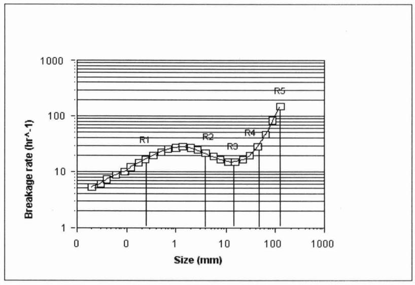
These rate curves exhibit a characteristic shape. The coarser (R5 and R4) rates relate to abrasive breakage while the finer rates R1 and R2 exhibit similar characteristics to those of coarse ball milling, ie. predominantly impact breakage. The pronounced dip in the rates at R3 is associated with the critical size which may limit mill throughput by building up to excessive levels. Typically it is in the 25-75mm range and varies with particular combinations of feed sizing, breakage characteristics and the magnitude of the breakage energy developed in the mill.
To determine the relationship between operating conditions and the breakage rate distribution, the breakage rates R1-R5 were regressed against operating conditions. The resultant equations were of the following form:
$$ Ln (R1) = (k_{11} + k_{12}Ln(R2) - k_{13}Ln(R3) + J_B (k_{14} - k_{15}F_{80}) - D_B)/S_b $$ (2)
$$ Ln (R2) = k_{21} + k_{22}Ln(R3) - k_{23}Ln(R4) - k_{24}F_{80} $$ (3)
$$ Ln (R3) = S_{a+}(k_{31} + k_{32} Ln(R4) - k_{33} R_r) / S_b $$ (4)
$$ Ln (R4) = S_b(k_{41} + k_{42} L_o(R5) + J_R(k_{43} - k_{44} F_{80})) $$ (5)
$$ Ln_{1}R5) = S_{a} + S_{b}(k_{51} + k_{52}F_{80} + J_{B}(k_{53} - k_{54}F_{80}) - 3D_{B}) $$ (6)
where
S, = rpm scaling factor
= Ln (simulated mill rpm123.6)
S, = fraction of critical speed scaling factor
= simulated mill fraction of critical speed10.75
D, = ball diameter scaling factor
= Ln (simulated ball diameterl90)
J, = % of total mill volume occupied by balls and associated voids
R, = recycle ratio
- - (tph recycled material -20+4mm) (tph new feed) + (tph recycled material -20+4mm)
F,, = 80% passing size of new feed (mm)
k, = regression coefficients
The regression coefficients for equations (2) - (6) are given in Table 2 and are based on the JKMRC's current data base. As more data are collected and our understanding of the various factors increases these coefficients are likely to be modified.
It can be seen from the equations that the finer size rates are functions of the rates of the coarser sizes. Hence R1 is a function of R2 and R3 etc. The rates can be considered as falling into 2 groups which represent the grinding media and product size fractions.
| Table 2: | Regression | Coefficients |
|---|
| j | k 1j | k 2j | \( k_{3j} \) | k 4j | k 5j |
|---|---|---|---|---|---|
| 1 | 2.504 | 4.68 | 3.14 | 1.057 | 1.894 |
| 2 | 0.397 | 0.468 | 0.402 | 0.333 | 0.014 |
| 3 | 0.597 | 0.327 | 4.632 | 0.171 | 0.473 |
| 4 | 0.192 | 0.0085 | 0.0014 | 0.002 | |
| 5 | 0.002 |
Hence the grinding media group contains the rates R4 and R5 (related to particles >30mm) the magnitude of which affect the throughput. The product group incorporates rates R1, R2 and R3 (related to particles < 30mm) and the magnitude of these affects the final product size. It is of particular note that the rates are interrelated in a complex manner and are best understood by plotting the entire breakage rate distribution.
Effect of Ball Load
The effect of changing ball load on the breakage rate distribution is illustrated in Figure 3.
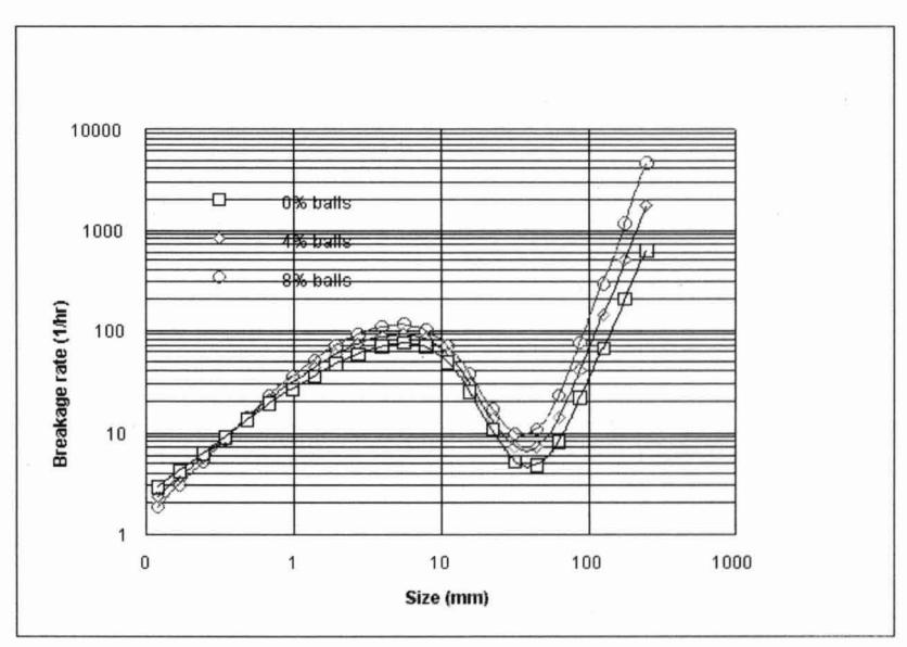
The resulting relationship is as expected in that by increasing the ball load the breakage rates increase at coarser sizes but reduce at finer sizes. This has the effect of predicting higher throughputs at coarser grinds as the ball load is increased. However, it is commonplace to operate at too high a ball charge often because of historical experience with softer, oxidised surface ore. As the ore becomes harder it may well be able to replace balls as grinding media for more power effective operation.
Effect of Feed Size (F80)
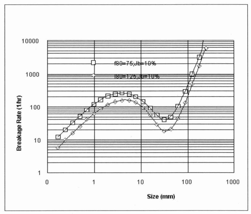
The effect of \( F_{80} \) was found to be the most difficult one to evaluate as it interacted with the ball charge level. At relatively high ball charges (10% or more) high \( F_{80} \) s were detrimental as evidenced by the reduction in the breakage rates illustrated in Figure 4.
However in the case of autogenous grinding the pattern is different. In this case a higher \( F_{80} \) promotes breakage in the coarser size fractions (Figure 5). This is to be expected when it is considered that in autogenous milling large rocks are required to break ore in the R5 size range (128mm).
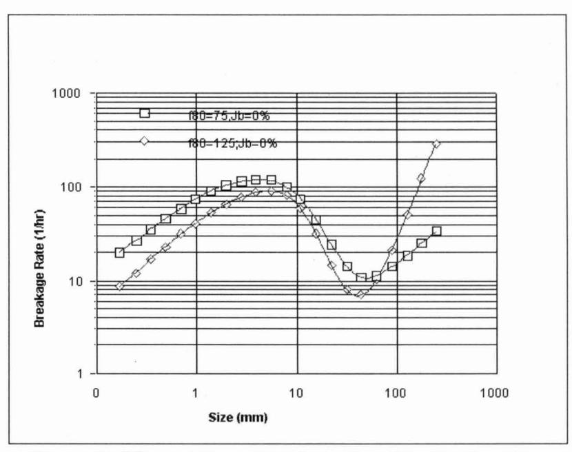
As the F80 increases, this will typically result in more coarse rocks in the charge able to break R5-size ore and hence R5 will increase. In SAG mills running with higher ball charges, the rock component of the grinding media plays a lesser role in dictating the breakage rate and contributes more to the rock 'burden' which has to be ground down. Feeds with higher F80's and hence more coarse feed rocks, can thus be expected to reduce the breakage Caution needs to be exercised, however, as it has been found that the F80 is not always a good indication of the feed size distribution. This is particularly noticeable with autogenous mills whose performance may fluctuate considerably yet maintain a reasonably constant F80. In such cases the distribution changes systematically with performance and that typically higher proportions of 25-50mm material in the feed result in lower feedrates, ie. less sub-grate size material is present in the feed and more near size material has to be broken.
In green-field design situations the question always arises as to what the expected AG/SAG mill feed size distribution will be. In the majority of existing installations the AGISAG mill is fed with prirnary crushed material, though rom or secondary crushed feed is used in some plants (Nelson et al, 1996; Needham & Folland, 1994). From the JKMRC data base the most popular gap setting in circuits using primary crushing only is of the order of 150mm (closed side setting) though in some cases up to 200mm is used. Crusher manufactures' grading curves typically give a P,, of 180mm for a 150mm css. However, for base metal and gold operations this appears to be an unrealistic estimate. Figure 6 shows the F,'s from over 100 mill feed sizings for 30 different mills which have been conducted by the JKMRC.
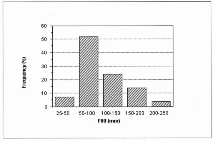
The modal F, is 75mm and is clearly much lower than the 180mrn determined from crusher manufacturers' data. The discrepancy has to do with the origins of manufacturers' data which typically derive from quarry applications and may be based on scalped feed to the crusher. Quarry operations endeavour to minimise the amount of fines produced and hence blasting practice reflects this requirement. The resultant coarse prirnary crusher feed therefore results in a coarse crusher product. In base metal and gold operations relatively large amounts of fines are produced and hence the primary crusher circuit product is typically much finer. To illustrate this effect Figure 7 shows a runof-mine (ie. uncrushed) size distribution from a gold operation which was determined by sizing approximately 85 tonnes of ore.
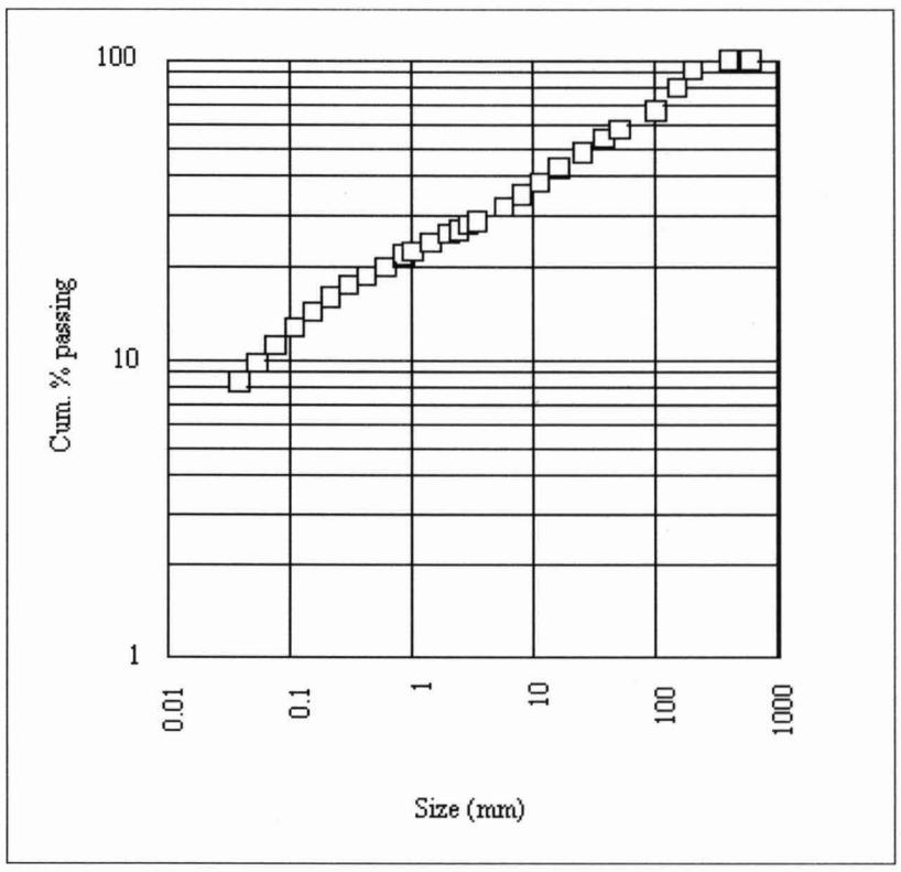
It can be seen that even in its uncrushed form the \( F_{80} \) is only 154mm and close to 20% of this material is already -1mm. By using the Andersen/Whiten crusher model (Andersen, 1989) it is possible to simulate the effect of crushing such a feed in a primary crusher set at 150mm (css). If the crusher feed is first scalped at 150mm the crusher would reduce the oversize to a \( P_{80} \) of 150mm ie. more in line with the crusher manufacturer's grading curves. On combining the crusher product with the scalper undersize an overall product \( P_{80} \) of 100mm is obtained ie. in line with the data in Figure 6.
For a given css, variations in the \( P_{80} \) will result from differences in ore hardness as well as variations in the blast (McKee, Chitombo & Morrell, 1995).
It has been found that the F, data correlate with the abrasion parameter (fa) which is a hardness indicator obtained from the SAGIAG mill laboratory tumbling test. Regression analysis of the data yielded the relationship:
$$ F_{80} = 71.3 - 28.4 \text{ Ln (t}_{a}) $$ (7)
A plot of the ta parameter vs primary crusher product (AGISAG F,) is shown in Figure 8.
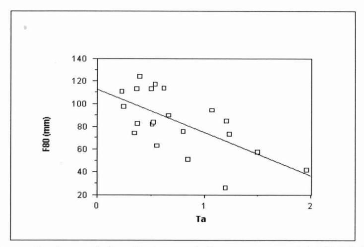
Scatter is obviously apparent though much of this can be explained by natural variations in crusher feed size distributions. To illustrate this Table 3 shows the results from repeat primary crusher product sizings from three different mines each crushing a nominally homogenous ore with a css of 150mm. The ores were chosen to give a wide range of t, values. The observed mean F,s as well as their standard deviations are shown, together with the predicted F,, using equation (7). It can be seen that the higher t, values coincide with the finer crusher products. The standard deviation is similar in each case being approximately 10% of the css. This gives rise to a 95% confidence interval of approximately i 30mm, which is in line with the scatter in Figure 8.
| ta |
No. Sur
VeYS |
Mean
Pa0 (mm) |
S.D. Pa,
(mm) |
Predicted
Pa0 (mm) |
|---|---|---|---|---|
| 0.36 | 9 | 113 | 15 | 100 |
| 0.68 | 5 | 92 | 17 | 82 |
| 1.5 | 12 | 57 | 17 | 59 |
Equation 7 was derived from crushers with closed settings of approximately 150mm. It can be extended to larger gap settings as follows:
$$ F_{80} $$ (mm) = {css - 78.7 - 28.4 ln (t a )} s.d. = 0.1 css. (8)
To test the validity of equation 8, 4 repeat surveys were conducted on a primary crusher with a nominal css of 200rnm. The ta parameter for the ore was 0.44. The survey results are shown in Table 4 together with the predicted F,, using equation 8. Reasonably close agreement was obtained.
| Observed | Predicted | |
|---|---|---|
| INO. Surveys |
4
I |
-
I |
| css (mm) | 200 | - |
| Mean F,,(mm) | 157 | 145 |
In a design scenario therefore, equation 8 is used to determine a likely F,, which in turn is used in the breakage rate equations (2)-(6).
Having chosen a F,, for the AGlSAG mill feed the question still arises as to what size distribution should be used.
Once again this will be influenced by blasting practice and ore type. To assist with this choice grading curves are extracted from the JKMRC data base to represent the ore in question, based on its hardness. Typical curves representing a coarse/hard ore, and a fine/soft ore are shown in Figure 9.
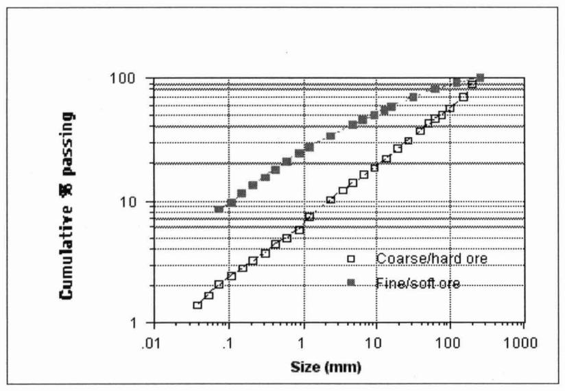
The majority of the size distributions in the data base fell in between these curves.
Effect of Recycle Load
Recycle loads broadly fall into 2 categories viz.:
- coarse recycles from trommels, vibrating screens and recycle crushers which typically comprise only -20 + 4mm material and have P80's of the order of 8 - 12mm,
- fine recycles from hydrocyclones and DSM screens which are predominantly - 4mm material and have P80's of the order of 0.2 - 0.5mm.
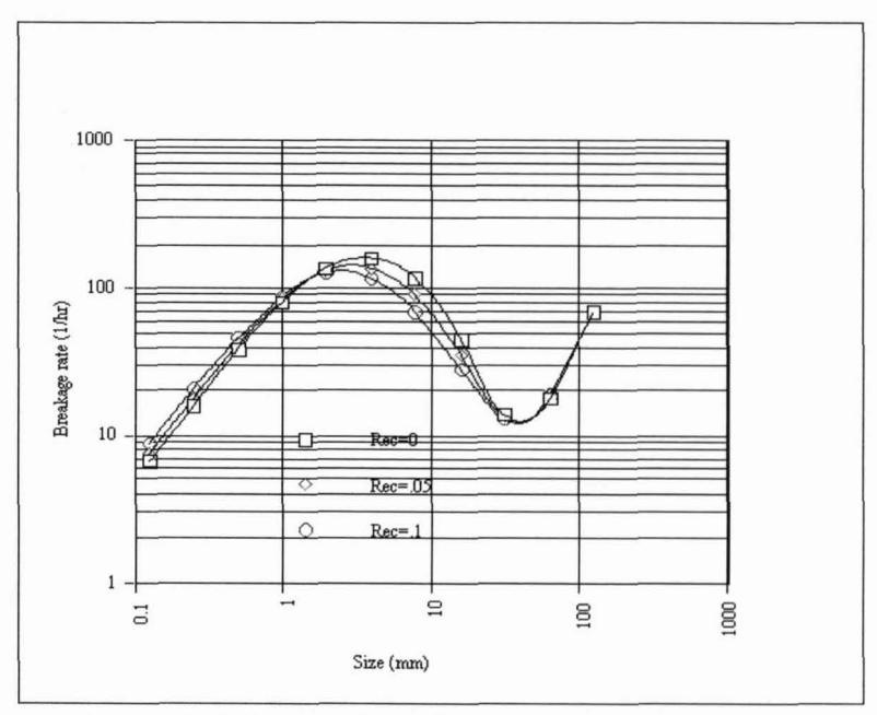
It has been found that the amount of recycled material in the -20 + 4mm size range is inversely related to the amount of breakage that this material is subjected to.
This can be explained if one considers that these rocks are broken by coarser rocks and balls whose frequency does not appreciably change with changes in recycle load. However as the amount of recycled -20 + 4mm rock increases, the amount of this size material in the load will increase. As the breakage rate in a given size class is related to the ratio of the number of coarser rocks and balls to the number of rocks in the given size class, then increasing the -20 + 4mm recycle will result in a drop in the breakage rate in this size range (R3 size = 16mm). The changes in the breakage rate distribution as the coarser recycle increases is illustrated in Figure 10. Interestingly, recycle of fine material ie. -4mm did not correlate with any of the breakage rates. This may be related to the breakage mode of this material which is believed to be dominated by attrition.
Effect of Speed
The breakage rate is related to the number of size reduction events per particle, per unit time and is hence a frequency.
This in turn must be related to the frequency with which the mill rotates (rpm). A scaling factor is therefore applied to account for changes in the rotational rate. For a given fraction of critical speed the rpm decreases with mill and hence this scaling factor will also change with mill diameter. All else being equal, therefore, a larger diameter mill will have a lower breakage rate than a smaller unit. However it is pointed out that the JKMRC model inherently scales on the basis of breakage energy which it relates to mill diameter. Therefore, whereas a larger diameter mill will have a lower breakage rate it will have a higher breakage energy.
In a given mill as the rpm changes, apart from the rotational rate, the shape of the grinding charge will also change in line with the fraction of critical speed (Morrell, 1996). Typically as the fraction of critical speed increases the charge is subjected to increased lift and hence impact breakage is enhanced. It is at the expense of attrition breakage which is normally associated with cascading motion and which is prevalent at lower speeds. To account for these effects a further scaling factor is applied which is based on the fraction of critical speed. Figure 11 illustrates the predicted changes in the breakage rate distribution as speed is changed.
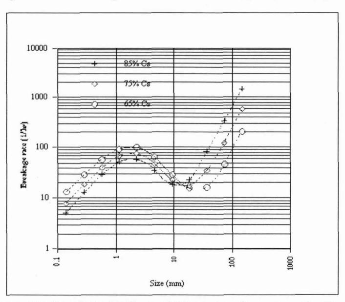
Effect of Ball Size
No significant dependence of the breakage rates on ball size was found in the pilot mill database. The sag model does account for ball size changes in terms of the energy provided during impact. It does this by changing the mean grinding media-size, which in turn changes the 'energy level' of the mill. This 'energy-level' term is used to determine the specific energy of impact. As the ball size is increased, therefore, the specific energy increases and hence for a given impact event a finer product size distribution occurs. However, as the ball size is increased the number of grinding media per tonne of charge will decrease. As the breakage rate is related to the number of impacts provided by the grinding media then a reduction in the breakage rate may be expected to occur. To account for this a ball scaling factor is used. Figure 12 illustrates the effect of the ball size correction factor on the breakage rate distribution.
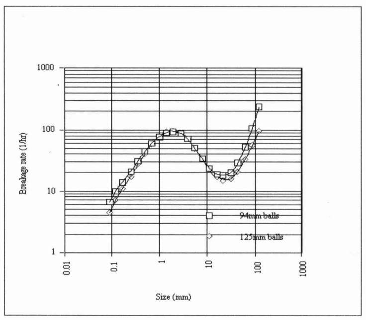
It should be emphasised that it is usually argued that a coarser ball size will give a higher throughput but with a coarser grind.
In practice, experiments with full scale mills are sometimes inconclusive and mill operators see little or no effect when ball size is experimented with. This may be due to the counter-effect of reduced numbers of balls providing higher breakage energies when increasing ball size. The model predicts such a response by increasing the breakage energy and reducing the breakage rate. In some instances the one effect may outweigh the other, in which case a response will be noted. Over some ranges of ball sizes, however, little or no effect will be seen.
PREDICTING AGISAG MILL PERFORMANCE
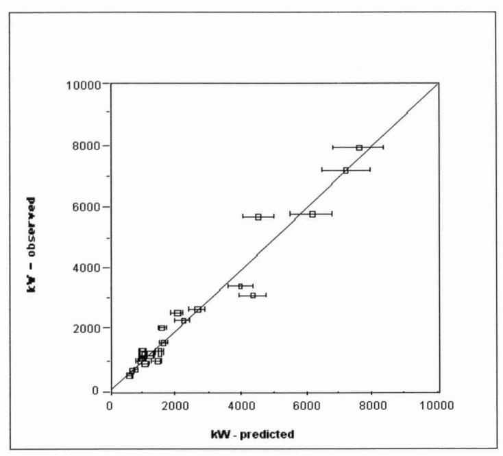
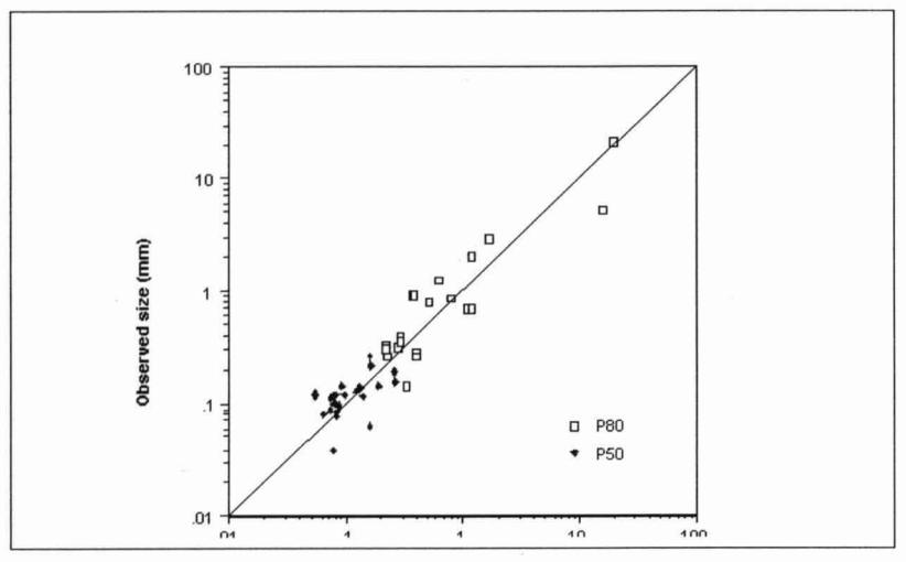
To determine the accuracy of the model in a design situation the performance of a number of full scale AGISAG mills which have been surveyed by the JKMRC was predicted, based solely on laboratory impact breakage and tumbling test results, coupled with mill design data. Details of the mills are given in Table 5. In each case the breakage rate distribution was determined using equations 2-6. The slurry hold-up - flowrate relationship was then calculated using equation 1. Using the measured feedrate and feed size distribution, the model was then used to predict both the mass of ore and water in the mill as well as the product size distribution. The simulated mass of ore and water in the mill was then used to predict the mill power using the JKMRC power draw model (Morrell, 1996). The observed and predicted power draws and associated 95% confidence intervals, and product size distributions as described by the P,, and P, are given in Figures 13 and 14 respectively.
It can be seen from Figure 13 that the observed and predicted power draws are well matched in most cases. One or two instances are apparent where the predictions are not quite as good as would be hoped. These are associated with autogenous operations where in practice it was found that even though the F,, remained constant, very large changes in mill performance were observed. This was due to the effect of feed size distribution for which the model only partly accounts. Figure 14 indicates that the product size distribution trends are followed reasonably well though scatter is apparent in the data. It is emphasised that these results are based solely on the breakage of rock samples of <50 kg. Where pilot data are available equations 2-6 can be fitted to generate a model which will predict full scale mill performance with an even higher degree of accuracy.
| Table 5: Will details | |
|---|---|
| Diameter (m) | AG/SAG |
| 7.05 | SAG |
| 7.73 | SAG |
| 5.08 | SAG |
| 4.35 | SAG |
| 3.9 | SAG |
| 4.05 | SAG |
| 9.56 | SAG |
| 9.56 | SAG |
| 6.49 | AG |
| 6.49 | AG |
| 7.11 | AG |
| 7.11 | AG |
| 6.5 | SAG |
| 6.5 | SAG |
| 6.51 | AG |
| 5.88 | AG |
| 9.4 | AG |
| 9.5 | AG |
| Diameter (m) 7.05 7.73 5.08 4.35 3.9 4.05 9.56 9.56 6.49 6.49 7.11 7.11 6.5 6.5 6.51 5.88 9.4 | |
Scaling Between Operating Conditions.
If a set of rates have been measured by plant survey and the ore breakage characteristics determined using the JKMRC's test methods, equations (2) - (6) can be used to estimate the effect of variations in ball load, mill speed etc. In this way optimisation strategies can be evaluated without recourse to costly and time consuming trial and error methods. JK breakage characterisation tests which include the more recently developed drop weight test, can be used on particles up to 90mm which provides an indication of ore competence at larger particle sizes.
These tests have become an accepted technique over the last decade with test facilities available at five laboratories world wide. The data base of breakage tests now covers more than 500 ore types. It should be noted that this technique only applies to materials which do break. It is not useful for "plastic" ores or those which change rapidly in water.
Using AGlSAG Product Size Distributions
The simulation model predicts a complete product size distribution. This line is almost never parallel with the feed size distribution. Hence traditional power methods based on product F80s are not valid. As these products typically contain more finished product that would be expected for a similar ball mill product, calculations based on P80 can be excessively conservative. If the circuit target product size is known, a simulated classifier can be used to remove this "extra" product and provide a realistic estimate of the effective feed sizing (and feed rate) to the next stage of size reduction.
CONCLUSIONS
A method has been developed for estimating grinding rates for the JK AGISAG mill model over a wide range of operating conditions. This allows the model to be used to aid in the design of AGlSAG mill circuits based solely on laboratory breakage tests and/or in conjunction with pilot mill data. Its application is seen to be for pre-feasibility studies, for limiting the size and cost of pilot mill programmes, designing full scale plants in conjunction with pilot mill results, and reducing risk when designing plants without pilot data.
REFERENCES
Ahlberg J H, Nilson, E N & Walsh, J L, 1967. The Theory of Splines and Their Applications. Mathematics in Science and Engineering, 38, Academic Press, New York and London
Andersen J S, 1989. Development of a Cone Crusher Model. M.Eng.Sc Thesis, University of Queensland.
Leung. K, Morrison R D & Whiten W J, 1987. 1987. An Energy Based Ore Specific Model for Autogenous and Semi-autogenous Grinding Mills. Copper 87, Santiago Chile.
McKee D J, Chitombo G P & Morrell S, 1995. The Relationship Between Fragmentation in Mining and Communition Circuit Throughput. Minerals Engineering , 8 , No. 11, pp.1266-1274.
Morrell, S. 1996. Power Draw of Wet Tumbling Mills and its Relationship to Charge Dynamics. Part I: A Continuum Approach to Mathematical Modelling of Mill Power Draw. Trans. Instn. Min.Metall, 105 , C43-53.
Morrell S & Stephenson I, 1996. Slurry Discharge Capacity of Autogenous and Semi-autogenous Mills and the Effect of Grate Design. Int. J. Miner. Process. (In press).
Morrell S, Finch W M, Kojovic T, Delboni H, Jr. 1995. Modelling and Simulation of Large Diameter Autogenous and Semi-Autogenous Mills. Int. J. Miner. Process. (In press).
Morrell S & Morrison R D,1989. Ore Charge, Ball Load and Material Flow Effects on an Energy Based SAG Mill Model. Presented SAG 1989, University of British Columbia. Editors. Mular & Agar.
Mutambo. J, 1993. Further Development of an Autogenous and Semi-autogenous Mill Model. M. Eng Sci. Thesis . Uni of Qld.
Needham T M & Folland G.V. 1994. Grinding Circuit Expansion at Kidston Gold Mine. Presented at SME Annual Meeting , Albuquerque, New Mexico. February 14 -17.