



The content on this page was automatically generated from the PDF publication document and may contain errors or inaccuracies. Please refer to the original PDF for the most accurate information.
Application of CCRD to modelling the effect of variables on the performance of the 3-product cyclone
D. P. Obeng, S. Morrell, T.J. Napier-Munn
Julius Kruttschnitt Mineral Research Centre, The University of Queensland, Isles Road, Indooroopilly, Qld. 4068, Australia
Abstract
Earlier work showed that the length of the second vortex finder had a substantial influence on the performance of the three-product cyclone. However, the statistical significance of this effect was not known. To determine the significance and model this effect, and those of the diameter of the second vortex finder, cyclone feed percent solids and inlet pressure, a process analysis and modelling technique that requires fewer tests and gives almost as much information as a three-level factorial design, namely the CCRD, was used.
The effects of the length and diameter of the second vortex finder, and the cyclone feed percent solids were found to be significant in most cases. The resultant model is also significant, predicts the experimental data well and can be used to estimate the response corresponding to operating conditions not included, but fall within the range of conditions in the experimental design.
Keywords: Classification; comminution; hydrocyclones; three-product cyclone, modelling
1. Introduction
The design, separation mechanism and some potential applications of the three-product cyclone have been described in detail by Obeng and Morrell (2003). The main features of the cyclone are depicted in Figure 1. As can be seen, the unit is a conventional hydrocyclone with a modified top cover plate and a second vortex finder inserted so as to generate three product streams - an Inner Overflow (INO), an Outer Overflow (OUO) and an underflow. The conventional and second vortex finders are referred to as Outer Vortex Finder (OVF) and Inner Vortex Finder (IVF) respectively. The unit uses a smaller spigot size than the conventional cyclone in order to create crowding and hindered settling conditions in the conical section. With the IVF length extending well into the cylindro-conical body, an additional exit is provided for the crowded particles. Hence the potential for underflow roping is reduced.
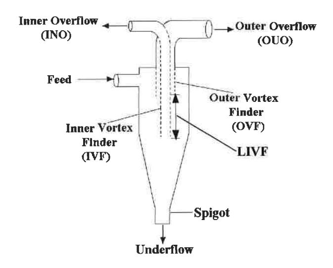
Work by Obeng and Morrell (2003) showed that the length of the second vortex finder had a substantial influence on the operational performance of the three-product cyclone. However, the statistical significance of this effect was not known. To determine the significance and model this effect, and those of the diameter of the second vortex finder, feed percent solids and inlet pressure, an appropriate experimental design technique had to be used.
The experimental design techniques commonly used for process analysis and modelling are the full factorial, partial factorial and central composite rotatable designs. A full factorial design requires at least three levels per variable to estimate the coefficients of the quadratic terms in the response model. Thus for the four independent variables mentioned above, 34 or 81 experiments, plus replications would have to be conducted. It has also been shown that a 3k factorial design estimates the coefficients of the squared terms in the model with relatively low precision (Box and Wilson, 1951). A partial factorial design requires fewer experiments than the full factorial. However, the former is particularly useful if certain variables are already known to show no interaction (Box and Hunter, 1961).
An effective alternative to the factorial design is the central composite rotatable design (CCRD), originally developed by Box and Wilson (1951) and improved upon by Box and Hunter (1957). The CCRD gives almost as much information as a three-level factorial, requires much fewer tests than the full factorial and has been shown to be sufficient to describe the majority of steady-state process responses (Cilliers et al., 1992; Crozier, 1992).
In this paper, the requirements for the CCRD and its application to the design of experiments, significance testing and modelling the effect of the four variables on the performance of the three-product cyclone are described.
2. REQUIREMENTS FOR THE CCRD
The number of tests required for the CCRD includes the standard \( 2^k \) factorial with its origin at the centre, 2k points fixed axially at a distance, say \( \beta \) , from the centre to generate the quadratic terms, and at least one test at the centre; where k is the number of variables. The axial points are often chosen such that they allow rotatability (Box and Hunter, 1957) which ensures that the variance of the model prediction is constant at all points equidistant from the design centre. Replicates of the test at the centre are very important as they provide an independent estimate of the experimental error. For four variables, the recommended number of tests at the centre is six (Box and Hunter, 1957). Hence the total number of tests required for the four independent variables is \( 2^4 + (2 \times 4) + 6 = 30 \) , which is at least, 51 experiments less than that required for a full factorial design. Figure 2 shows the CCRD and the co-ordinates for k = 4 factors.
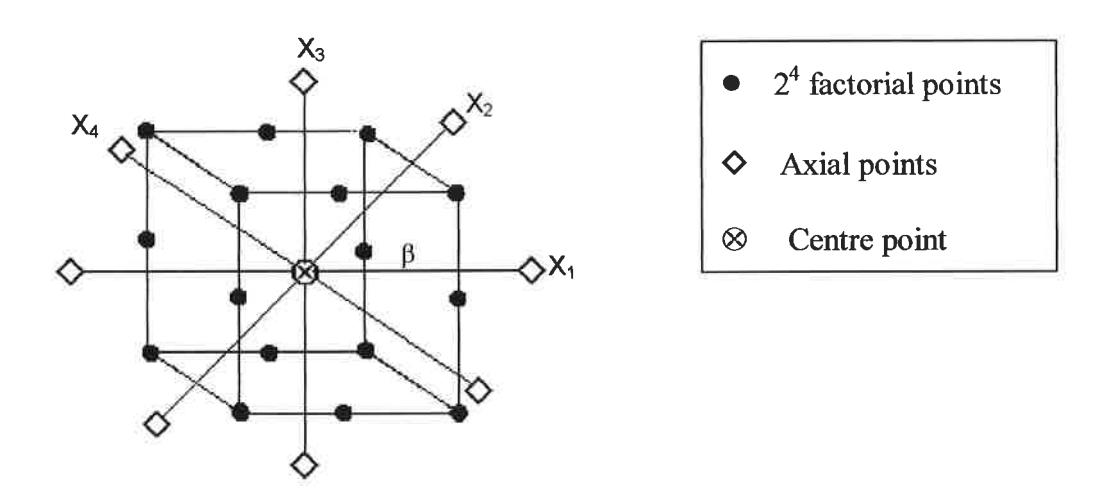
Once the desired range of values of the variables are defined, they are coded to lie at \( \pm 1 \) for the factorial points, (0,0) for the centre points and \( \pm \beta \) for the axial points. The codes are calculated as shown in Table 1.
| Code | Actual value of variable |
|---|---|
| - β | X min |
| - 1 | $$ \frac{\left(\mathbf{x}_{\max} + \mathbf{x}_{\min}\right)}{\left(\mathbf{x}_{\max} - \mathbf{x}_{\min}\right)} $$ |
| \( 2 2\alpha \) | |
| 0 | \( (x_{\text{max}} + x_{\text{min}}) \) |
| 2 | |
| + 1 | \( \left(\mathbf{x}_{\max} + \mathbf{x}_{\min}\right)_{+} \left(\mathbf{x}_{\max} - \mathbf{x}_{\min}\right) \) |
| \( 2 \) \( 2\alpha \) | |
| + β | X max |
\( x_{max} \) and \( x_{min} \) = maximum and minimum values of x respectively; \( \alpha = 2^{k/4} \) ; k = number of variables
When the response data are obtained from the test work, regression analysis is carried out to determine the coefficients of the response model \( (a_1, a_2, ..., a_n) \) , their standard errors and significance. In addition to the constant \( (a_0) \) and error \( (\epsilon) \) terms, the response model incorporates:
- Linear terms in each of the variables \( (x_1, x_2, ..., x_n) \)
- Squared terms in each of the variables \( (x_1^2, x_2^2, ...x_n^2) \)
- First order interaction terms for each paired combination \( (x_1x_2, x_1x_3, ..., x_{n-i}x_n) \)
Thus for the four variables under consideration, the response model is:
$$ a_{0} + a_{1}x_{1} + a_{2}x_{2} + a_{3}x_{3} + a_{4}x_{4} + a_{11}x_{1}^{2} + a_{22}x_{2}^{2} + a_{33}x_{3}^{2} + a_{44}x_{4}^{2} + a_{12}x_{1}x_{2} + a_{13}x_{1}x_{3} + a_{14}x_{1}x_{4} + a_{23}x_{2}x_{3} + a_{24}x_{2}x_{4} + a_{34}x_{3}x_{4} + \varepsilon $$ (1)
A detailed analysis of variance (ANOVA) is also carried out to determine the statistical significance of the linear, square and interaction terms in the response model.
3. EXPERIMENTAL DESIGN
To provide data to determine the statistical significance and model the effect of the variables on the performance of the three-product cyclone via the CCRD approach, the range of values for each variable was defined as follows:
Length of IVF below the OVF (LIVF): 50 - 585 mm
Diameter of IVF (DIVF): 35 - 50 mm Cyclone feed percent solids: 30 - 60 % Cyclone inlet pressure: 80 - 130 kPa
Using the relationships in Table 1, the actual levels of the variables for each of the thirty experiments in the design matrix were calculated. Table 2 gives the coded and actual levels of the variables.
| ) | Coded level of variables | Actual levels of variables | |||||||
|---|---|---|---|---|---|---|---|---|---|
| 1 | Test | Pressure | % Solids | LIVF | DIVF | Pressure | % Solids | LIVF | DIVF |
| No | 1100000 | , 0 10 0 11 11 | (kPa) | (w/w) | (mm) | (mm) | |||
| 1 | -1 | -1 | -1 | -1 | 92.5 | 37.5 | 183.8 | 38.8 | |
| 2 | +1 | ÷1 | -1 | e=1 | 117.5 | 37.5 | 183.8 | 38.8 | |
| 3 | -1 | +1 | -1 | -1 | 92.5 | 52.5 | 183.8 | 38.8 | |
| 4 | -1 | -1 | +1 | -1 | 92.5 | 37.5 | 451.3 | 38.8 | |
| 5 | -1 | -1 | -1 | +1 | 92.5 | 37.5 | 183.8 | 46.3 | |
| 6 | +1 | +1 | =1 | -1 | 117.5 | 52.5 | 183.8 | 38.8 | |
| Factorial | 7 | +1 | -1 | +1 | -1 | 117.5 | 37.5 | 451.3 | 38.8 |
| Points | 8 | +1 | -1 | -1 | +1 | 117.5 | 37.5 | 183.8 | 46.3 |
| Polits | 9 | -1 | +1 | +1 | -1 | 92.5 | 52.5 | 451.3 | 38.8 |
| 10 | -1 | +1 | -1 | +1 | 92.5 | 52.5 | 183.8 | 46.3 | |
| 11 | =1 | -1 | +1 | +1 | 92.5 | 37.5 | 451.3 | 46.3 | |
| 12 | +1 | +1 | +1 | -1 | 117.5 | 52.5 | 451.3 | 38.8 | |
| 13 | +1 | +1 | -1 | +1 | 117.5 | 52.5 | 183.8 | 46.3 | |
| 14 | +1 | -1 | +1 | +1 | 117.5 | 37.5 | 451.3 | 46.3 | |
| 15 | -1 | +1 | +1 | +1 | 92.5 | 52.5 | 451.3 | 46.3 | |
| 16 | +1 | +1 | +1 | +1 | 117.5 | 52.5 | 451.3 | 46.3 | |
| 17 | -β | 0 | 0 | 0 | 80.0 | 45.0 | 317.5 | 42.5 | |
| 18 | +β | 0 | 0 | 0 | 130.0 | 45.0 | 317.5 | 42.5 | |
|
Axial
Points |
19 | 0 | -β | 0 | 0 | 105.0 | 30.0 | 317.5 | 42.5 |
| 20 | 0 | +β | 0 | 0 | 105.0 | 60.0 | 317.5 | 42.5 | |
| 21 | 0 | 0 | -β | 0 | 105.0 | 45.0 | 50.0 | 42.5 | |
| 22 | 0 | 0 | +β | 0 | 105.0 | 45.0 | 585.0 | 42.5 | |
| 23 | 0 | 0 | 0 | -β | 105.0 | 45.0 | 317.5 | 35.0 | |
| 24 | 0 | 0 | 0 | +β | 105.0 | 45.0 | 317.5 | 50.0 | |
| Centre | 25 | 0 | 0 | 0 | 0 | 105.0 | 45.0 | 317.5 | 42.5 |
| 26 | 0 | 0 | 0 | 0 | 105.0 | 45.0 | 317.5 | 42.5 | |
| 27 | 0 | 0 | 0 | 0 | 105.0 | 45.0 | 317.5 | 42.5 | |
| 28 | 0 | 0 | 0 | 0 | 105.0 | 45.0 | 317.5 | 42.5 | |
| Points | 29 | 0 | 0 | 0 | 0 | 105.0 | 45.0 | 317.5 | 42.5 |
| 30 | 0 | 0 | 0 | 0 | 105.0 | 45.0 | 317.5 | 42.5 | |
4. TEST CYCLONE, MATERIAL, RIG, PROCEDURE, SAMPLE AND DATA ANALYSES
The three-product cyclone used for the tests was a 150-mm unit with dimensions of fixed components given in Table 3. The test material was a mixture of magnetite (s.g. = 4.7) and silica (s.g. = 2.7) in which the former comprised approximately 18 % by weight. The 80 % and 20 % passing sizes were 203 and 13 \( \mu \) m respectively. The test rig, procedure and sample analysis were the same as described by Obeng and Morrell (2003). Because the CCRD requires exact positioning of the test points as far as is practicable (Cilliers et al., 1992), the exact levels of the variables given in Table 2 were used. The particle size distributions were measured on the Malvern Mastersizer. The experimental data were mass balanced and used subsequent for analysis.
| Cyclone diameter | 150 mm |
|---|---|
| Inlet diameter | 36 mm |
| Diameter of OVF | 60 mm |
| Spigot diameter | 25 mm |
| Cone angle | 100 |
Dimensions of other cyclone components are given in Table 2.
5. RESULTS AND DISCUSSION
The mass balanced experimental results are summarised in Table A1 in Appendix 1. Results of the regression analysis showing the effect of all the terms (both significant and non-significant) in the response surface model (Equation 1) have been reported (Obeng, 2003). The results in Tables 4-9 show the effect and significance of the individual linear and/or square and/or interaction terms obtained by stepwise refitting the response surface model using only the terms that are significant at greater than or equal to 90 % confidence level, i.e \( P(t) \le 0.1 \) . Note, however, that in some cases the linear terms, irrespective of their significance, had to be included as the software used required that for every interaction or square term included in the refit, the corresponding linear term must be included. The graphs in Figures 3-8 which are simulations from the response surface model describe the effect of the variables on the performance of the three-product cyclone. The explanations for the trends in Figures 3-8 have been given by Obeng (2003).
5.1 EFFECT OF VARIABLES ON SIZE DISTRIBUTION IN OUO
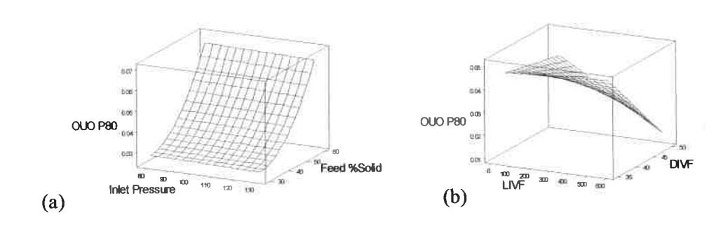
The influence of the four variables on P80 in the OUO is depicted in Figure 3 while Table 4 gives the effect, along with the significance of the individual terms. The P(t) values in the table show that the effects of the feed percent solids squared and feed percent solids-IVF length interaction terms are significant at 92.4 % (i.e. 1-0.076) and 90 % (i.e. 1-0.100) confidence levels respectively. Note that the linear feed percent solids and LIVF terms are included in this case as a requirement of the software used.
| Term | Coefficient | SE of Coefficient | t | P(t) | ||
|---|---|---|---|---|---|---|
| Constant | 2.67 x 10 -2 | 0.048763 | 0.547 | 0.589 | ||
| Feed % solids | -1.37 x 10 -3 | 0.001998 | -0.683 | 0.501 | ||
| LIVF | 1.01 x 10 -4 | 0.000075 | 1.355 | 0.188 | ||
| Feed % solids* Feed % solids | 4.0 x 10 -5 | 0.000021 | 1.848 | 0.076 | ||
| Feed % solids* LIVF | -3.0 x 10 -6 | 0.000002 | -1.686 | 0.100 | ||
| \( R^2 = 72.5\% \) \( R^2 \) (Adjusted) = | 68.2% | *** | ||||
| ANOVA | ||||||
| Source | DF | Seq SS | Adj SS | Adj MS | F | P(F) |
| Regression | 4 | 0.002861 | 0.002861 | 0.000715 | 16.52 | 0.000 |
| Linear | 2 | 0.002593 | 0.000127 | 0.000064 | 1.47 | 0.250 |
| Square | 1 | 0.000145 | 0.000148 | 0.000148 | 3.42 | 0.076 |
| Interaction | 1 | 0.000123 | 0.000123 | 0.000123 | 2.84 | 0.104 |
| Residual Error | 25 | 0.001083 | 0.001083 | 0.000043 | ||
| Total | 29 | 0.003943 |
Substituting the coefficients in Table 4 in the response surface Equation 1, we obtain the regression equation for P80 in the OUO as:
$$ OUOP80 = 2.67 \times 10^{-2} - 1.37 \times 10^{-3} \times FS + 1.01 \times 10^{-4} LIVF + 4 \times 10^{-5} FS^{2} - 3 \times 10^{-6} FS \times LIVF $$ (2)
where the symbols/acronyms have their meanings given in the nomenclature at the end of this chapter.
The P(F) values from the ANOVA in Table 4 show that the linear, square and interaction terms of Equation 2 are significant at 75 %, 92.4 % and 89.6 % confidence levels respectively, with regression Equation 2 being significant at greater than 99.9 % confidence level.
5.2 EFFECT OF VARIABLES ON SIZE DISTRIBUTION IN INO
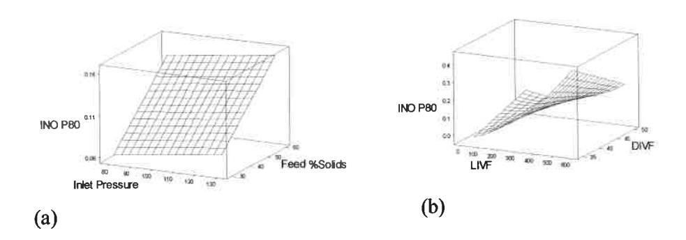
Figure 4 shows the influence of the variables on P80 in the INO while Table 5 shows that the effects of the cyclone feed percent solids, LIVF and DIVF are significant at 98.6, 99.9 and 94.2 % confidence levels respectively.
| Term | Coefficient | SE of Coefficient | t | P(t) | ||
|---|---|---|---|---|---|---|
| Constant | 1.56 x 10 -2 | 0.103587 | 0.151 | 0.882 | ||
| Feed % solids | 2.8 x 10 -2 | 0.001057 | 2.627 | 0.014 | ||
| LIVF | 5.1 x 10 -4 | 0.000059 | 8.585 | 0.000 | ||
| DIVF | -4.2 x 10 -3 | 0.002115 | -1.979 | 0.058 | ||
| \( R^2 = 76.5\% \) \( R^2(Adjusted) = \) | 73.8% | |||||
| ANOVA | ||||||
| Source | DF | Seq SS | Adj SS | Adj MS | F | P(F) |
| Regression | 3 | 0.127724 | 0.127724 | 0.042575 | 28.20 | 0.000 |
| Linear | 3 | 0.127724 | 0.127724 | 0.042575 | 28.20 | 0.000 |
| Residual Error | 23 | 0.039249 | 0.039249 | 0.001510 | ||
| Total | 29 | 0.166973 |
Substituting the values of the coefficients in Table 5 in Equation 1 gives the regression equation for the P80 in the INO as:
$$ INOP80 = 1.56 \times 10^{-2} + 2.78 \times 10^{-3} FS + 5.10 \times 10^{-4} LIVF - 4.20 \times 10^{-3} DIVF $$ (3)
where the symbols/acronyms have their meanings given in the nomenclature at the end of this chapter.
From the ANOVA in Table 5, the linear terms, as well as the regression Equation 3 are significant at greater than 99.9 % confidence level.
5.3 EFFECT OF VARIABLES ON FEED VOLUMETRIC FLOWRATE
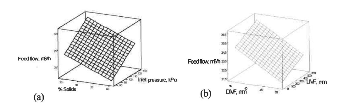
Figure 5 shows the effect of the four variables on cyclone feed volumetric flowrate. The P(t) values in Table 6 show that the effects of the inlet pressure and feed percent solids are significant at greater than 99.9 % confidence level while that of the DIVF is significant at 96.7 % confidence level. The effect of LIVF does not appear in the table as it is not significant in this case.
| Term | Coefficient | SE of Coefficient | t | P(t) | ||
|---|---|---|---|---|---|---|
| Constant | 27.23 | 5.35843 | 5.081 | 0.000 | ||
| Inlet pressure | 0.14 | 0.02792 | 4.867 | 0.000 | ||
| Feed % solids | -0.19 | 0.04652 | -4.144 | 0.000 | ||
| DIVF | -0.21 | 0.09307 | -2.252 | 0.033 | ľ | |
| \( R^2 = 63.9\% \) \( R^2 \) (Adjust | ed) = 59.7% | |||||
| ANOVA | ||||||
| Source | DF | Seq SS | Adj SS | Adj MS | F | P(F) |
| Regression | 3 | 134.419 | 134.419 | 44.8064 | 15.33 | 0.000 |
| Linear | 3 | 134.419 | 134.419 | 44.8064 | 15.33 | 0.000 |
| Residual Error | 26 | 76.010 | 76.010 | 2.29235 | ||
| Total | 29 | 210.429 |
Data used for the analysis are given in Table A1 in Appendix 1; the meanings of the acronyms are given in the Nomenclature at the end of this chapter.
Substituting the coefficients of the terms in Table 6 in the response surface model (Equation 1), we obtain the regression equation for the feed volumetric flowrate \( (Q_f) \) as:
where the symbols/acronyms have their meanings given in the nomenclature at the end of this chapter.
The P(F) values in Table 6 show that the linear term and the overall regression Equation 4 are significant at greater than 99.9 % confidence level.
5.4 EFFECT OF VARIABLES ON WATER RECOVERY TO OUO
Figure 6 depicts the influence of the variables on water recovery to the OUO while Table 7 shows that the effects of the cyclone feed percent solids, LIVF, DIVF, DIVF squared and feed percent solids-DIVF interaction terms are significant at 97.7, 99.9, 99.6, 99.9 and 95.5 % confidence levels respectively.
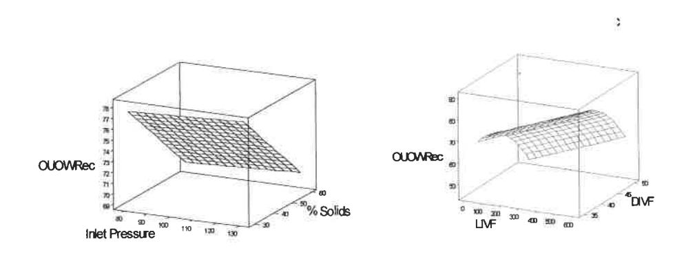
Substituting the coefficients of the terms in Table 7 in Equation 1, the regression equation for water recovery to the OUO is:
OUOW Re $$ c = -22.86 - 1.92 \times FS + 0.03 LIVF + 7.91 DIVF - 0.13 DIVF^2 + 0.04 FS \times DIVF $$ (5)
where the symbols/acronyms have their meanings given in the nomenclature at the end of this chapter.
The analysis of variance in Table 7 shows that the linear and square terms are both significant at greater than 99.9 % confidence level while the interaction term is significant at 95.5 % confidence level. The regression Equation 5 is also significant at greater than 99.9 % confidence level.
| Term | Coefficient | SE of Coefficient | t | P(t) | ||
|---|---|---|---|---|---|---|
| Constant | -22.86 | 61.2854 | -0.373 | 0.712 | ||
| Feed % solids | -1.92 | 0.7916 | -2.428 | 0.023 | ||
| LIVF | 0.03 | 0.0032 | 9.963 | 0.000 | ||
| DIVF | 7.91 | 2.4934 | 3.172 | 0.004 | ||
| DIVF * DIVF | -0.13 | 0.0276 | -4.783 | 0.000 | ||
| Feed % solids* DIVF | 0.04 | 0.0189 | 2.113 | 0.045 | ||
| \( R^2 = 93.2\% \) \( R^2 \) (Adjusted | d) = 91.8% | |||||
| ANOVA | ||||||
| Source | DF | Seq SS | Adj SS | Adj MS | F | P(F) |
| Regression | 5 | 1428.14 | 1428.14 | 285.628 | 66.08 | 0.000 |
| Linear | 3 | 1309.35 | 532.927 | 177.642 | 41.09 | 0.000 |
| Square | 1 | 99.49 | 98.884 | 98.884 | 22.88 | 0.000 |
| Interaction | 1 | 19.30 | 19.300 | 19.300 | 4.46 | 0.045 |
| Residual Error | 24 | 103.75 | 103.746 | 4.323 | ||
| Total | 29 | 1531.89 |
5.5 EFFECT OF VARIABLES ON WATER RECOVERY TO INO
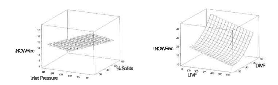
The influence of the variables on water recovery to the INO is illustrated in Figure 7. Table 8 shows that aside from the effect of the cyclone feed percent solids which is significant at 90 % confidence level, the effects of the LIVF, DIVF and DIVF squared terms are all significant at greater than 99.9 % confidence level.
Substituting the coefficients of the terms in Table 8 in Equation 1, the regression equation for water recovery to the INO is:
INOW Re $$ c = 228.73 - 0.11FS - 0.03LIVF - 10.99DIVF + 0.15DIVF^2 $$ (6)
where the symbols/acronyms have their meanings given in the nomenclature at the end of this chapter.
The analysis of variance in Table 8 shows that the linear, square terms and the regression Equation 6 are significant at greater than 99.9 % confidence level.
| Term | Coefficient | SE of Coefficient | T | P(t) | ||
|---|---|---|---|---|---|---|
| Constant | 228.73 | 57.6067 | 3.971 | 0.001 | ||
| Feed % solids | -0.11 | 0.0655 | -1.637 | 0.100 | ||
| LIVF | -0.03 | 0.0037 | -7.648 | 0.000 | ||
| DIVF | -10.99 | 2.7135 | -4.051 | 0.000 | ||
| DIVF* DIVF | 0.15 | 0.0319 | 4.623 | 0.000 | ||
| \( R^2 = 89.8\% \) \( R^2 \) (Adjust | ed) = 88.2% | |||||
| ANOVA | ||||||
| Source | DF | Seq SS | Adj SS | Adj MS | F | P(F) |
| Regression | 4 | 1277.45 | 1277.449 | 319.362 | 55.15 | 0.000 |
| Linear | 3 | 1153.68 | 449.128 | 149.709 | 25.85 | 0.000 |
| Square | 1 | 123.77 | 123.765 | 123.765 | 21.37 | 0.000 |
| Residual Error | 25 | 144.76 | 144.763 | 5.791 | ||
| Total | 29 | 1422.21 |
5.6 EFFECT OF VARIABLES ON WATER RECOVERY TO UNDERFLOW
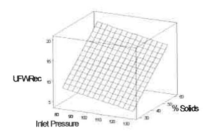
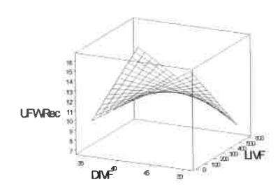
The effect of the variables on water recovery to the underflow is depicted in Figure 8 with Table 9 showing that the effects of the LIVF and cyclone feed percent solids-LIVF interaction terms both being significant at greater than 99.4 % confidence level. Note that the cyclone feed percent solids term appears in this case as a requirement of the software used.
| Term | Coefficient | SE of Coefficient | t | P(t) | ||
|---|---|---|---|---|---|---|
| Constant | 20.2661 | 8.25823 | 2.454 | 0.021 | ||
| Feed % solids | -0.1630 | 0.18253 | -0.893 | 0.380 | ||
| LIVF | -0.0780 | 0.02475 | -3.150 | 0.004 | ||
| Feed % solids* LIVF | 0.0017 | 0.00055 | 3.036 | 0.005 | ||
| \( R^2 = 64.4\% \) \( R^2 \) (Adjusted) = | 60.3% | |||||
| 700 | ANOVA | |||||
| Source | DF | Seq SS | Adj SS | Adj MS | F | P(F) |
| Regression | 3 | 225.084 | 225.084 | 75.028 | 15.71 | 0.000 |
| Linear | 2 | 181.062 | 212.493 | 106.246 | 22.24 | 0.000 |
| Interaction | 1 | 44.022 | 44.022 | 44.022 | 9.21 | 0.005 |
| Residual Error | 26 | 124.211 | 124.211 | 4.777 | ||
| Total | 29 | 349.295 |
Substituting the coefficients of the terms in Table 9 in Equation 1, the governing regression equation for water recovery to the underflow is:
UFW Re $$ c = 20.27 - 1.63 \times 10^{-1} FS - 7.80 \times 10^{-2} LIVF + 1.70 \times 10^{-3} \times FS \times LIVF $$ (7)
where the symbols/acronyms have their meanings given in the nomenclature at the end of this chapter.
The analysis of variance in Table 9 shows that the linear and interaction terms are significant at 99.9 % and 99.5 % confidence levels respectively, the regression Equation 7 being significant at greater than 99.9 % confidence level.
6. CORRELATION BETWEEN PREDICTED AND OBSERVED RESPONSES
Figure 9 shows the correlation between the model-predicted and observed responses for Equations 2 to 7. As can be seen from the figure and the \( R^2 \) values in Tables 4-9, the equations fit the experimental data reasonably well. The analyses of variance (ANOVA) in Tables 4-9 also show that the linear, square and/or interaction terms, as the case may be, are generally significant, the resultant regression equation in each case being significant at greater than 99.9 % confidence level, i.e. \( P(F) \approx 0.00 \) .
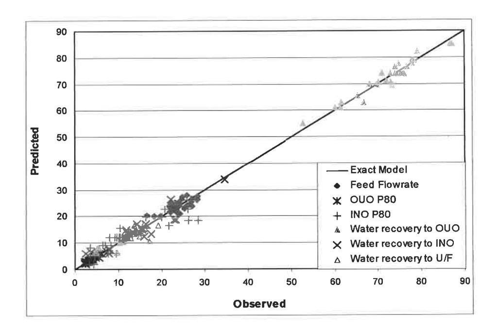
The above attributes show that the influence of the variables as described by the regression Equations 2-7 is significant. Hence they can be used to estimate the response for variations in IVF length and diameter, cyclone inlet pressure and feed percent solids not included in the experimental design but fall within the range of conditions given in Section 3.
It is worth noting that the trends obtained for the influence of feed percent solids on water recovery to the product streams and IVF length on size distribution in the overflows are consistent with those obtained from tests with other feed materials (Obeng, 2003; Obeng and Morrell, 2003).
7. CONCLUSIONS
The Central Composite Rotatable Design (CCRD) has been successfully applied to the design of an experimental program to establish the general process trends, determine the statistical significance and model the effect of IVF length and diameter, inlet pressure and feed percent solids on the performance of the three-product cyclone. The number of experiments required for the CCRD was 51 less than that required for a three-level full factorial design.
The effects of the length and diameter of the second vortex finder, and the cyclone feed percent solids were found to be significant in most cases. The resultant model is also significant, predicts the experimental data well and can be used to estimate the response corresponding to operating conditions not included, but fall within the range of conditions in the experimental design.
The trends obtained for the influence of IVF length on size distribution in the overflows and feed percent solids on water recovery to the product streams were consistent with those obtained from tests with other feed materials.
NOMENCLATURE
DIVF: Cyclone inner vortex finder diameter (m)
INO Inner overflow stream IVF Inner vortex finder
LIVF: Length of inner vortex finder (m) F20: feed 20 % passing size (mm)
F80: feed 80 % passing size (mm)
FS: feed percent solids
OUO: Outer overflow stream OVF: Outer vortex finder
P: Cyclone inlet pressure (kPa)
Qf: feed flowrate (m3/h)
\( R_f \) : Water recovery to underflow (%)
ACRONYMS FOR TABLES 4-9:
Adj MS: Adjusted mean square Adj SS: Adjusted sum of squares ANOVA: Analysis of variance
DF: Degrees of freedom
F: F- statistic
P(F): Probability value of F- statistic indicating level of significance P(t): Probability value of t- statistic indicating level of significance
R2: Coefficient of determination
R2(Adjusted): Coefficient of determination adjusted for degrees of freedom
SE of Coefficient: Standard error of coefficient
Seq SS: Sequential sum of squares
t: t- statistic
ACKNOWLEDGMENTS
The authors are thankful to the sponsors of the JKMRC/AMIRA P9L/M Mineral Processing projects for the financial and logistics support.
REFERENCES
- Obeng, D. P., 2003. The three-product cyclone separation performance, potential applications and modelling. PhD Thesis, JKMRC, The University of Queensland, Brisbane, Australia.
- Obeng, D. P. and Morrell, S., 2003. The JK three-product cyclone performance and potential applications, International Journal of Mineral Processing, Vol. 69, pp. 129-142.
- Box, G.E.P. and Wilson, K.B., 1951. On the experimental attainment of optimum conditions. J. Royal Stat. Soc. , Series B, Vol 13, 1-45.
- Box, G.E.P. and Hunter, J.S., 1957. Multi-factor experimental design for exploring response surfaces. Annals of Math. Stats. , Vol 28, 195-241.
- Box, G.E.P. and Hunter, W.G, 1961. The 2k-p Fractional Factorial Designs Part I & II. J. Technometrics, Vol 3, 311-458.
- Cilliers, J.J., Austin, R.C. and Tucker, J.P., 1992. An evaluation of formal experimental design procedures for hydrocyclone modelling. Proc. 4th Int. Conf. on Hydrocyclones , Southampton, ("Hydrocyclones: analysis and applications"), Ed. Svarovsky, L. and Thew, M.T., Kluwer Academic Publishers, 31-49.
- Crozier, R.D., 1992. Flotation Theory, Reagents and Ore Testing. Pergamon Press, New York.
- Napier-Munn, T.J., 2000. The central composite rotatable design. JKMRC, The University of Queensland, Brisbane, Australia. Pp. 1-9.
APPENDIX 1
Table A1 - Mass balanced experimental response data
| Feed flowrate, m /n | P80OUO, mm | P80INO, mm | OUOWRec, % | INOWRec, % | UFWRec, % | |
|---|---|---|---|---|---|---|
| Test | 0.031 | 0.035 | 76.7 | 11.8 | 11.5 | |
| 1 | 24.1 | 0.046 | 74.0 | 15.7 | 10.4 | |
| 2 | 25.8 | 0.033 | 0.063 | 73.1 | 12.4 | 14.5 |
| 3 | 23.4 | 0.056 | 0.285 | 86.7 | 7.8 | 5.5 |
| 4 | 26.4 | 0.042 | 66.6 | 22.2 | 11.2 | |
| 5 | 22.2 | 0.031 | 0.033 | 70.2 | 17.7 | 12.1 |
| 6 | 22.2 | 0.059 | 87.2 | 8.0 | 4.8 | |
| 7 | 28.2 | 0.042 | 0.263 | 61.5 | 27.4 | 11.1 |
| 8 | 24.6 | 0.026 | 0.043 | 78.3 | 2.4 | 19.4 |
| 9 | 22.0 | 0.049 | 0,26 | 24.0 | 15.9 | |
| 10 | 18.2 | 0.049 | 0.075 | 60.1 | 22.9 | 5.2 |
| 11 | 25.2 | 0.024 | 0.155 | 71.9 | 7.8 | 14.2 |
| 12 | 23.7 | 0.047 | 0.207 | 78.0 | 23.8 | 14.9 |
| 13 | 22.8 | 0.047 | 0.095 | 61.3 | 4.5 | |
| 14 | 28.3 | 0.022 | 0.166 | 72.1 | 23.4 | 13.8 |
| 15 | 19.7 | 0.037 | 0.165 | 69.8 | 16.5 | 12.3 |
| 16 | 23.3 | 0.041 | 0.201 | 73.4 | 14.3 | 13.8 |
| 17 | 16.5 | 0.038 | 0.079 | 71.0 | 15.2 | 10.4 |
| 18 | 28.1 | 0.035 | 0.109 | 75.1 | 14.5 | 9.6 |
| 19 | 27.0 | 0.022 | 0.034 | 74.8 | 15.6 | |
| 20 | 24.3 | 0.073 | 0.218 | 68.1 | 15.9 | 16.0 |
| 21 | 23.9 | 0.055 | 0.056 | 65.2 | 22.8 | 11.9 |
| 22 | 21.7 | 0.031 | 0.259 | 79.0 | 3.7 | 17.3 |
| 23 | 26.8 | 0.046 | 0.104 | 77.9 | 10.7 | 11.4 |
| 24 | 23.3 | 0.025 | 0.07 | 52.6 | 34.6 | 12.8 |
| 25 | 24.1 | 0.036 | 0.104 | 75.6 | 13.1 | 11.3 |
| 26 | 24.1 | 0.035 | 0.102 | 72.9 | 14.9 | 12.2 |
| 24.1 | 0.04 | 0.11 | 74.4 | 13.5 | 12.1 | |
| 27 | 24.1 | 0.04 | 0.104 | 76.2 | 12.1 | 11.7 |
| 28 | 24.9 | 0.037 | 0.097 | 74.0 | 14.6 | 11.4 |
|
29
30 |
24.5 | 0.037 | 0.093 | 72.9 | 15.2 | 11.9 |