



The content on this page was automatically generated from the PDF publication document and may contain errors or inaccuracies. Please refer to the original PDF for the most accurate information.
DEM VALIDATION FOR A SCALE MODEL SAG MILL
Paul W. Cleary 1, Rob Morrison 2, Steve Morrell 2 1CSIRO Division of Mathematical and Information Sciences, Private Bag 10, Clayton South MDC, Clayton, Vic, 3169. Australia. 2 Julius Kruttschnitt Mineral Research Center, Isles Rd, Indooroopilly, Qld, 4068, Australia
ABSTRACT
Simulations of a scale model SAG mill have been performed to closely match earlier experiments performed at JKMRC. Quantitative comparison of the charge distributions, the shoulder and toe positions between the experiments and the different DEM models employed allows the effect of different modelling assumptions to be evaluated. Comparisons are made for a given fill level and three mill speeds for three different liner profiles. These comparisons demonstrate that traditional two-dimensional DEM simulations using circular particles under-predict shoulder and toe positions by around 10° and show that particle shape makes an important contribution to the shape of the charge profile. Importantly they demonstrate that full three-dimensional modelling is able to quantitatively capture the real dynamics found in the experimental mill.
INTRODUCTION
DEM has been used to model many industrial applications over the past decade. Of specific interest here is the modelling of ball mills by Mishra and Rajamani (1992, 1994), Inoue (1995), Cleary (1998a, 2001b), Datta et.al. (1999) and SAG mills by Rajamani and Mishra (1996) and Cleary (2001a) and others. DEM has been used for many other applications with example given by Ristow (1994) and Cleary (1998b).
Modelling of SAG mills by discrete element methods (DEM) is already leading to improved understanding of charge dynamics, and offers the potential to improve mill design and control. This could lead to reduced downtime, increased mill efficiency, increased throughput, lower costs and lower energy consumption.
Validation of the predictions made by DEM is a critical part of understanding the effect of various modelling assumptions and for separating more accurate DEM variants from less accurate ones. One such example of validation by Cleary and Hoyer (2000) demonstrated excellent agreement between DEM simulation and experiment (both in terms of the charge motion and the power draw) for a centrifugal mill. Here we continue the validation effort by comparing the predictions of a range of DEM models with experimental photographs of a scale model SAG mill by Ward (1992). Detailed quantitative comparison is made using the angular positions of the shoulder and toe of the charge.
THE DISCRETE ELEMENT METHOD
DEM simulation involves following the motion of every particle in the flow and modelling each collision between the particles and between the particles and their environment (e.g. the mill liner). Industrial applications place heavy demands on the geometrical capabilities of DEM codes, particularly for three-dimensional geometries. In our DEM code, any two-dimensional cross section can be constructed using an appropriate number of line segments, circular segments or discs. This gives essentially unrestricted geometric capability. In three-dimensions, boundary objects can be constructed by either extruding two dimensional cross sections or by importing triangular finite-element surface meshes. Such meshes can be produced using any reasonable mesh generator from solid models generated in suitable CAD packages. This provides enormous flexibility in specifying three-dimensional environments with which the particles interact.
The particles are currently modelled as spheres in three-dimensions and by discs or super-quadrics in two-dimensions. Super-quadrics are defined by the equation
where the power N determines the blockiness or angularity of the resulting particle and A determines the aspect ratio. Aspect ratios of up to 12:1 and angularity factors of up to 20 can be used. Arbitrary size, shape and density distributions can be specified for the particles.
The general DEM methodology and its variants are well established and are described in review articles by Barker (1994), Campbell (1990) and Walton (1994). Here we use a conventional implementation that is described in more detail in Cleary (1998a&b). Briefly, the particles are allowed to overlap and the amount of overlap 2x, and normal 2x and tangential 2x relative velocities determine the collisional forces via a contact force law. We use a linear spring-dashpot model. For more complex models see Schäfer (1996) and Walton (1994). The normal force
consists of a linear spring to provide the repulsive force and a dashpot to dissipate a proportion of the relative kinetic energy. The maximum overlap between particles is determined by the stiffness \( k_n \) of the spring in the normal direction. Typically, average overlaps of 0.1-0.5% are desirable, requiring spring constants of the order of \( 10^7 \) N/m in two dimensions and \( 10^6 \) N/m in three dimensions. The spring constants required to achieve these overlap target overlaps are lower in three dimensions than in two dimensions, since the force exerted on particles is proportional to their masses, and the mass of a spherical particle is much smaller than that of a cylinder of unit length. The normal damping coefficient \( C_n \) is chosen to give the required coefficient of restitution? (defined as the ratio of the post-collisional to pre-collisional normal component of the relative velocity), and is given in Cleary (1998b). The tangential force is given by
where the vector force \( F_t \) and velocity \( v_t \) are defined in the plane tangent to the surface at the contact point. The integral term represents an incremental spring that stores energy from the relative tangential motion and models the elastic tangential deformation of the contacting surfaces, while the dashpot dissipates energy from the tangential motion and models the tangential plastic deformation of the contact. The total tangential force \( F_t \) is limited by the Coulomb frictional limit \( ?F_{n,} \) , at which point the surface contact shears and the particles begin to slide over each other. The discrete element algorithm has three main stages:
-A search grid is used to periodically build a near-neighbour interaction list that contains all the particle pairs that are likely to experience a collision in the short term. Using only particle pairs in this list reduces the force calculation to an O(M) operation, where M is the total number of particles. Industrial simulations with 500,000 particles are now possible in reasonable times on current single processor workstations.
- -The forces on each pair of colliding particles and/or boundary objects are evaluated in their local reference frame using the spring-dash pot model and then transformed into the simulation frame of reference.
- All the forces and torques on the particles and objects are summed and the resulting equations of motion are integrated. Time integration is performed using a second-order predictor-corrector scheme and typically uses between 15 and 25 time steps to integrate accurately each collision. This leads to small time steps (typically 10-4 to 10-6 s depending on the controlling length and time).
Quantitative predictions of boundary stresses, wear rates and distributions, collision forces, energy spectra, power consumption, torques and flow rates, sampling statistics, mixing and segregation rates and many other quantities can be made from the information available in DEM simulations. For more details on the simulation method and on the data analysis see Cleary (1998c).
MILL GEOMETRY AND CONFIGURATIONS FOR COMPARISON
The experimental mill had an internal diameter of 592 mm and a depth of 200 mm. It was a 1:10 scale model of the Alcoa SAG mill at Pinjarra. Three different liners were used, 1) C-Noranda lifters, 2) ICAL lifters and 3) smooth liner. For both the first two cases there are 44 lifter plates arranged circumferentially around the mill interior. Both the Noranda and the ICAL lifters were 18 mm high and 42 mm long with a 5 mm deep base plate. The effective face angles were 30° and 12° respectively. The direction of rotation for the mill was counter-clockwise in order to match the experiments.
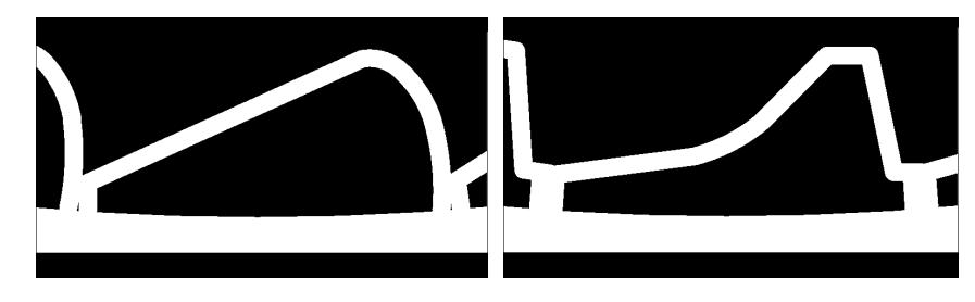
The experiments were conducted using a basalt ore with specific gravity of 2.84. The size distribution was chosen to match exactly the complete experimental charge (see Ward, 1992). For the Noranda lifters, fill levels of 35% and 45% by volume were used in both the experiments and simulations for three speeds, being 65%, 75% and 95% of the critical speed of 56 rpm. In the 2D simulations the particle shapes were either circular or super-quadric with blockiness between 2.1 and 5.0 and aspect ratios between 0.4 and 1.0. Such a choice gives a plausible range of particle shapes and is used to demonstrate the effect of such shape on the shoulder and toe positions. In 3D, the particles are modelled as spheres.
For all the calculations presented here the coefficient of restitution used was e = 0.3 and the friction coefficient is µ = 0.75. These are reasonable values for dry rock materials such as basalt ores.
MODEL OPTIONS AND COMPUTATIONAL TIMES
For such a mill configuration there are essentially three options for the type of geometric model:
- 1. 2D model where the particles are cylinders that are constrained to move in the XY plane. This is the most common type of model because of its much smaller computational size. We use two variants of this a) using traditional circular particles and b) super-quadrics.
- 2. 3D slice model a slice of a 3D mill model is used with periodic boundaries in the axial direction. This allows 3D particles to be used but restricts the computational size of the problem that depends then on the thickness of the slice.
- 3. A full 3D model the full 3D particle and mill geometries are used, including end wall effects on the axial direction. This is the largest, most expensive but most realistic of the models.
STREAK PICTURES AND SHOULDER AND TOE MEASUREMENT
DEM predictions of particle flows are normally presented as instantaneous snapshots showing the locations, sizes, shapes and orientations of all the particles. Figure 2a shows particles in a typical 2D DEM flow for this scale model mill with a fill level of 35% and a speed of 75% critical. The flow pattern involves a cataracting stream consisting predominantly of smaller particles due to radial segregation and a free surface that is bi-linear in shape with the charge cascading down from the shoulder to the toe region.
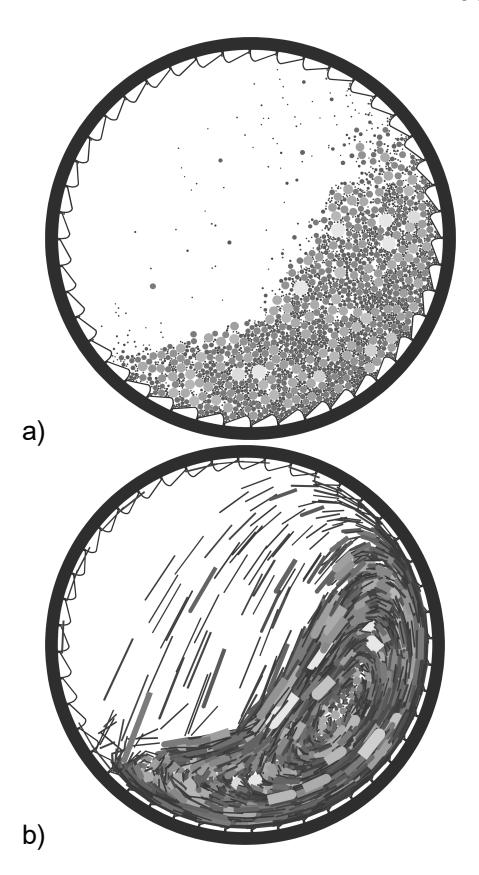
The use of a camera with a finite shutter opening duration (between 1/20 and 1/30) leads the real particles to record streaks on the photograph showing their trajectories during the time the film is exposed (Ward, 1992). These streaks contain useful information about the recent history of each particles motion. They also make the shoulder and toe locations much more clearly identifiable. Importantly, the streaks in the cascading region fill in this region making it look solid with the free surface appearing higher.
It is important to represent the DEM flow in a manner that is as consistent with this as possible.
The positions of each particle in the DEM simulation were recorded at the start and end of each photographic period (of 1/25 s) and these points were connected by lines with thicknesses equal to the diameter of the particle. This streak then represents the area that the particle has covered during the recording period. Figure 2b shows the streak picture that corresponds to the snapshot shown in Figure 2a. This computational streak picture captures most of the essential features of the photographic streaks. The shoulder and toe positions are clearly defined. Streaks at similar distances from the vortex center visually join together form rings that are centered on the stationary point in the middle of the charge.
The shoulder and toe locations are the primary quantitative information available in Ward (1992) for comparison with the simulations. We use the same conventions for specifying angles, measuring in a counterclockwise direction from the 3 o'clock location. The shoulder angle is the angle associated with the highest point reached by the charge in the shoulder region of the mill. The toe angle is the highest point reached by the bulk of the charge at the base of the cascading free surface. Significant care was taken in the identification of the shoulder and toe angles, particularly in 3D to ensure that they were as close as possible to that measured in the experiments. To provide more robust estimates of the shoulder and toe angles for comparison with the experiments we have also averaged the limits of these angles for ensembles of 25 streak pictures at intervals of 0.25 s in 2D and for ensembles of 10 streak pictures at intervals of 0.1 s in 3D. The average upper and lower limits are then representative of the variation in the behaviour of the mill charge and errors introduced by the subjective nature of the shoulder and toe identification are substantially reduced. Thee errors are estimated to be less than 1-2 degrees.
COMPARISON OF DEM MODELS FOR 45% FILL AND SPEED 65%
Figure 3 shows typical streak pictures for the four types of DEM model and the experimental photograph for a fill level of 45% and a speed of 65% critical.
The overall flow patterns are qualitatively similar for all the pictures in Figure 3 shown on the next page. The charge rises up to the shoulder and most cascades down a free surface to the toe, with a modest cataracting stream that lands well short of the toe position. There are, however, important differences in the details.
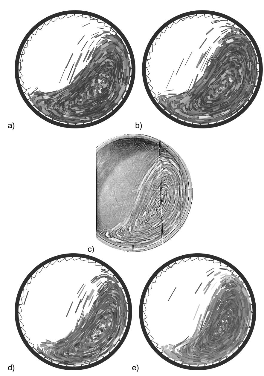
Comparing the 2D circular model with the experiment we see that the toe is much too large and its position is too high and the shoulder position is also too low. Also, the free surface is more of a circular arc than the yingyang shape in the experiment. The use of non-circular particles, increases the strength of the charge microstructure and leads to a higher shoulder and a lower and slightly smaller toe, but the shape of the free surface remains different to that of the experiment.
The 3D slice model includes the effects of the three dimensionality of the particle microstructure on the charge shear strength. This has little effect on the shoulder position, but has a marked effect on the toe with a substantial reduction in the size and a significant increase in the toe angle. The shape of the free surface improves somewhat, but is still more similar to the 2D case than the experiment.
The full 3D model simulates the entire axial length of the mill and includes the compressive and frictional effects of the end walls. This gives very close agreement with the experiment. The toe has been lowered further and is now only marginally bigger that the experimental one. The shoulder has also moves higher to around the correct level and the free surface now has the correct ying-yang shape of the experiment and is in the correct position.
This comparison allows us to understand the penalty for each of the modelling assumptions that is traditionally made for DEM modelling of mills and establishes that if all the effects are included the charge behaviour can be predicted very well.
FULL 3D DEM vs EXPERIMENT - THREE DIFFERENT SPEEDS
Figure 4 on the next page shows a comparison of the full 3D DEM predictions with the experiments for three mill speeds and a fill level of 35% for the Noranda lifters. At 65% critical the charge sits high up on the right with a high shoulder and a small toe. There is only a small amount of cataracting material with most cascading down the ying-yang shaped free surface. There is a high degree of correspondence between the DEM prediction and the experiment in all the key areas. For a 75% mill speed the charge moves higher giving larger shoulder and toe angles and a larger amount of curvature to the upper part of the free surface. There is still only a modest amount of cataracting. The DEM prediction again closely captures the essential features of the charge distribution. For a 95% critical speed, most of the charge is thrown in a cataracting stream and a free surface is visible within the vortex.
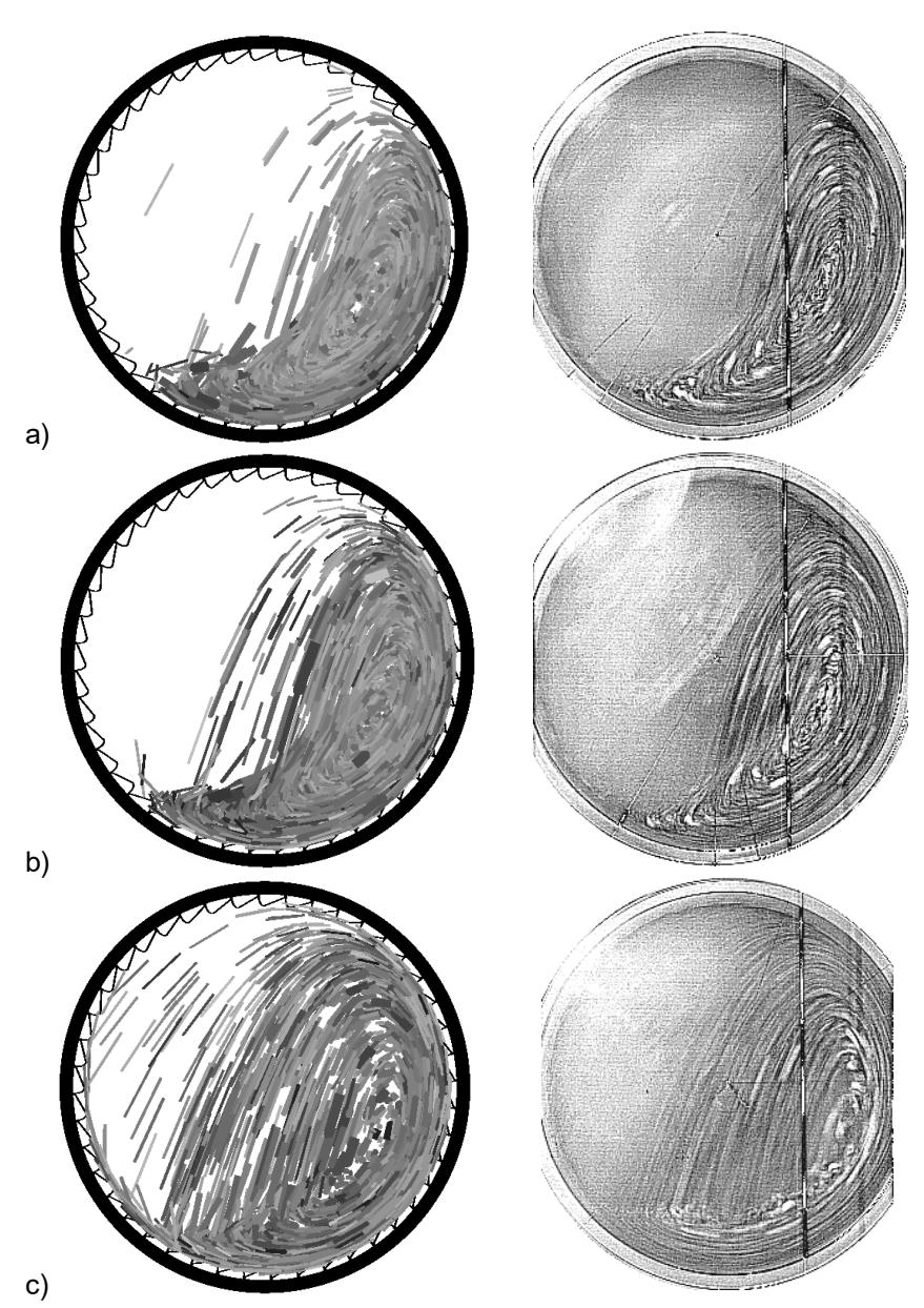
Most of the charge is thrown on high trajectories to land between the vortex center and the toe. The DEM prediction again captures these important features.
2D VS 3D DEM FOR DIFFERENT LINERS
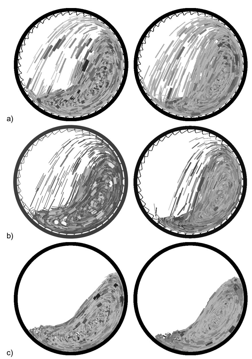
Figure 5 on the next page shows the DEM predictions of the charge location for three different liners with the 2D circular particle results (left) and full 3D (right).
The flow patterns for the ICAL and Noranda lifters are quite similar, with the main difference being the larger amount of cataracting material thrown well past the toe for the ICAL case. This is to be expected since the ICAL lifter has a much steeper effective face angle that the Noranda lifters. Otherwise the shoulder and toe positions and the free surface shape are similar for these two liners. The charge shape for a smooth liner is however, clearly different. The charge is much more slumped with an extremely clearly defined free surface and absolutely no cataracting material.
For both the ICAL and the Noranda lifter the difference between the 2D and 3D models are very similar. In the 3D case, the shoulder is higher leading to the cataracting stream being thrown further and the toe is much smaller and is much further to the right. The free surface in both cases acquires much more curvature near the top leading to the characteristic ying-yang shape observed in the experiments. For the smooth liner the charge shape is very similar for the two DEM models. The main differences for this case are really just a reflection of the modestly lower actual fill level in the 3D case resulting from a slightly lower bulk density for the charge.
QUANTITATIVE COMPARISON OF SHOULDER AND TOE POSITIONS
Quantitative comparison of the key shoulder and toe positions is made possible by the use of ensemble averages for both the DEM predictions and the experiments from Ward (1992). Tables 1 and 2 (see page following Figure 5) show the variation of shoulder and toe angles with the type of DEM model used for the Noranda lifters for six combinations of fill level and mill speed. All four DEM model variants produce qualitatively similar flow patterns, but with important differences in the shoulder and toe positions, that can be summarised as:
- The 2D circular model consistently under-predicts the shoulder and toe locations by around 10°. This occurs because the circular particle microstructure is weaker than it should be and fails more easily producing a more slumped charge.
- The inclusion of particle shape increases the shear strength of the charge microstructure leading to higher shoulder locations (by around 3 -5°). Particle shape seems to have little effect on the toe location.
- The 3D slice model includes the locking effects of particles in 3D which also increases the strength of the microstructure. This has a much larger effect on the predicted location of the toe (increasing it by 6-8° for lower mill speeds)
- The full 3D model also includes the very strong frictional and compressive support of the end wall effects. The motion of the walls helps lift the charge higher, while the axial compression strengthens the charge, leading to higher and much more accurate predictions of the shoulder and toe positions and of the free surface shape.
| Fill | Speed | Exp | 2D-C | 2D-NC | 3D slice | Full 3D |
| 35% | 65% | 46-50 | 37-43 | 41-45 | 35-42 | 41-44 |
| 35% | 75% | 50-56 | 41-44 | 45-50 | 40-46 | 45-49 |
| 35% | 95% | 69-72 | 59-70 | 59-70 | 66-73 | 68-78 |
| 45% | 65% | 51-55 | 44-47 | 47-50 | 43-46 | 45-49 |
| 45% | 75% | 59-63 | 49-53 | 55-59 | 50-54 | 55-59 |
| 45% | 95% | 82-86 | 66-78 | 71-83 | 70-84 | 75-88 |
| Table 2: Toe positions for the Noranda lifters |
|---|
| Fill | Speed | Exp | 2D-C | 2D-NC | 3D slice | Full 3D |
|---|---|---|---|---|---|---|
| 35% | 65% | 228-232 | 218-220 | 219-222 | 225-228 | 228-231 |
| 35% | 75% | 232-238 | 219-221 | 219-223 | 225-229 | 226-231 |
| 35% | 95% | 206-224 | 218-224 | 219-227 | 208-227 | 198-232 |
| 45% | 65% | 223-223 | 208-210 | 209-212 | 218-220 | 222-225 |
| 45% | 75% | 220-230 | 210-213 | 212-215 | 219-221 | 219-225 |
| 45% | 95% | 194-222 | 209-218 | 202-213 | 187-226 | 185-223 |
Tables 3 and 4 show the shoulder and toe positions for a fill level of 35% and a speed of 75% critical for all three liners when using three of the DEM models. Firstly, we compare the shoulder positions for the ICAL and Noranda lifters for each of the DEM models and see a small but consistent difference that results from the much steeper face angle of the ICAL lifter. This is largest for the full 3D model. This shows that the shoulder position is only a weak function of the steepness of the lifter face.
| Lifter type | 2D-C | 2D-NC | Full 3D | Exp |
|---|---|---|---|---|
| ICAL | 41-45 | 46-51 | 49-52 | 57-64 |
| Noranda | 41-44 | 45-50 | 45-49 | 50-56 |
| Smooth | 32-34 | 37-40 | 30-32 | 48-53 |
| Lifter type | 2D-C | 2D-NC | Full 3D | Exp |
|---|---|---|---|---|
| ICAL | 218-222 | 220-224 | 225-231 | 237-238 |
| Noranda | 219-221 | 219-223 | 225-229 | 232-238 |
| Smooth | 216-218 | 218-221 | 227-229 | 227-229 |
For each of the three models though, there is little sign of any sensitivity in the toe position to the details of the lifter. The smooth liner gives consistently much lower shoulder positions, but only slightly lower toe angles. This reflects the much straighter shape of the free surface with much more of the material sitting in lower positions in the mills. The changes with the different DEM models are quite consistent for all three lifter types, with the exception of the shoulder position for the full 3D model of the smooth liner. The inclusion of particle shape increases the shoulder position, on average by 4-6°. The full 3D results for the shoulder position are more variable, with the ICAL lifter producing an 8° increase, the Noranda lifter 4-5° degree increase and the smooth liner a decrease of around 5°. For the toe positions, the inclusion of shape in 2D leads to, on average a 2° increase, while the full 3D model leads to increases of between 6° and 11°.
CONCLUSION
Predictions of the shoulder and toe locations have been made for several combinations of mill fill and speed and for three different liners using four different types of DEM models. The 2D circular model consistently under-predicts the shoulder and toe positions by around 10°, with the charge being much more slumped and the toe much larger than in reality.
The inclusion of particle shape consistently increases the shoulder angle by 3-6°, but affects the toe only marginally. For the Noranda lifter, the 3D slice model produced a significant improvement in the toe size and location. The predictions of the full 3D model are quantitatively the closest to those of the experiments with good matching of shoulder and toe locations, and close agreement on the shape of the free surface and the size of the toe.
REFERENCES
Barker, G. C., 1994, "Computer simulations of granular materials", Granular Matter: An interdisciplinary approach , Ed. Anita Mehta, Springer-Verlag, NY.
Campbell, C. S., 1990, "Rapid Granular Flows", Annual Rev. Fluid Mech. , Vol. 22, pp. 57-92.
Cleary, P. W., 1998a, "Predicting charge motion, power draw, segregation, wear and particle breakage in ball mills using discrete element methods'', Minerals Engineering, Vol. 11, pp. 1061-1080.
Cleary, P. W., 1998b, "Discrete Element Modelling of Industrial Granular Flow Applications", TASK. Quarterly - Scientific Bulletin , Vol. 2, pp. 385-416.
Cleary, P. W., 2001a, ``Modelling Comminution Devices using DEM'', Int. J. for Numer. Anal. Meth. Geomechan ., Vol. 25, pp. 83-105.
Cleary, P. W., 2001b, ``Charge behaviour and power consumption in ball mills: Sensitivity to mill operating conditions, liner geometry and charge composition'', to appear: Int. J. Min. Processing .
Cleary, P. W., and Hoyer, D., 2000, ``Centrifugal mill charge motion: comparison of DEM predictions with experiment'', Int. J. Min. Proc ., Vol. 59, pp. 131-148.
Datta, A., Mishra, B. K., and Rajamani, R. K., 1999, "Analysis of power draw in ball mills by discrete element method", Can. Metall. Quart ., Vol. 38, pp. 133-140.
Inoue, T., and Okaya, K., 1995, "Analysis of grinding actions of ball mills by discrete element method", Proc. XIX Int. Min. Proc. Congress , Vol. 1, Society for Mining, Metallurgy and Exploration, pp. 191-196.
Mishra, B. K., and Rajamani, R. J., 1992, The discrete element method for the simulation of ball mills, App. Math. Modelling , Vol. 16, pp. 598- 604.
Mishra, B. K., and Rajamani, R. K., 1994, Simulation of charge motion in ball mills. Part 1: Experimental verifications, Int. J. Mineral Processing, Vol. 40, pp. 171--186.
Rajamani, R. K., and Mishra, B. K., 1996, "Dynamics of ball and rock charge in sag mills", Proc. SAG 1996 , Department of Mining and Mineral Process Engineering, University of British Columbia.
Ristow, G. H., 1994, Granular Dynamics: A review about recent Molecular Dynamics Simulations, Annual Rev. of Comp. Phys ., Vol. 1, pp. 275-308.
Schäfer, J., Dippel, S., and Wolf, D. E., 1996, "Force schemes in simulation of granular material", J. Physique I France , Vol. 6, pp. 5.
Ward, B. K, 1992, "Optimisation of the design of lifter profiles in grinding mills", B.Sc. Metallurgy (Hons) Thesis, University of Queensland (unpublished).
Walton, O. R., 1994, "Numerical simulation of inelastic frictional particleparticle interaction", Chapter 25, Particulate two-phase flow , Ed. M. C. Roco, pp. 884-911.