



The content on this page was automatically generated from the PDF publication document and may contain errors or inaccuracies. Please refer to the original PDF for the most accurate information.
GRINDING MILLS - HOW TO ACCURATELY PREDICT THEIR POWER DRAW
S.Morrell
JKMRC, Isles Road, Indooroopilly, Queensland, 4068
ABSTRACT
The first 90 years of the last century generated a considerable volume of technical literature on the subject of grinding mill power and its prediction. It is therefore surprising that during this time there were no published models for predicting grinding mill power draw which were validated using a wide range of comprehensive industrial scale data.
Notwithstanding this lack of data, the majority of models placed limited emphasis on the internal dynamics of mills and relied on simple assumptions which considered the charge to take up a fixed position and shape.
Laboratory based studies (Liddell, 1986) and industrial data (Morrell, 1993) showed that these assumptions did not hold over a wide range of operating conditions, and brought into doubt the ability of the (then) existing models to accurately predict grinding mill power draw. Furthermore no model treated AG,SAG and ball mills as a single class of devices whose power draw could be predicted with the same equations.
Through a detailed investigation of the charge dynamics, coupled with a large data base of industrial mill power draws this situation was rectified by the end of the century by which time a model had been developed and validated which accurately predicted the power draw of all wet tumbling mills. This paper describes this model and reviews some of the earlier attempts at mill power modelling.
Keywords: power, milling, grinding, modelling
INTRODUCTION
The early 1900's saw the beginnings of published papers which tackled the problem of what influenced the power draw of tumbling mills and what equations (models) were suitable for predicting power draw. This interest continued for the rest of the 20th century and the literature contains many papers that attempted to satisfactorily answer these questions. A common and disappointing theme in the majority of them, however, is the distinct lack of suitable experimentally derived power draw data. This deficiency consequently limited the practical application of many of the attempts at modelling mill power draw. Prior to the early 1990's some limited data on the power draw of grinding mills in the literature can be found, but as Harris et al (1985) remarked they are "... too frequently unusable simply because one or more essential variables have been omitted". The absence of published results from vigorous experimental testing of the various models has resulted in a general lack of evaluation of the validity of assumptions and hypotheses that such models contain. Harris et al (1985) however, did make some efforts in attempting to evaluate the performance of various power prediction equations and in so doing further developed a semi-empirical one of their own. However, in using manufacturers' published data, which themselves were undoubtedly generated by proprietary equations of unproven validity, they most likely succeeded in generating little more than a consensus of the various errors in these models.
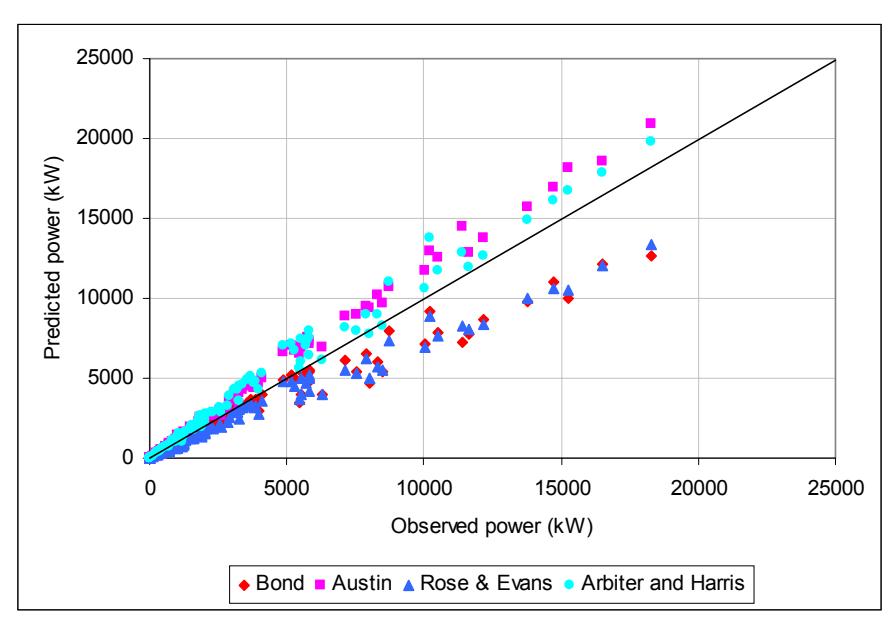
Notwithstanding this lack of quality data, the majority of models placed limited emphasis on the internal dynamics of mills and relied on simple assumptions which considered the charge to take up a fixed position and shape. As early as 1986 (Liddell, 1986) showed that these assumptions did not hold over a wide range of operating conditions, and brought into doubt the ability of the (then) existing models to accurately predict grinding mill power draw. This conclusion was supported by Morrell (1993) who evaluated a number of models using a large data base of power draws (Figure 1).
In this paper the factors which need to be addressed in order that tumbling mill power draw can be accurately predicted are discussed. A power model that incorporates each of these factors is described and its ability to predict power draw accurately is demonstrated.
HISTORICAL PERSPECTIVE
Before discussing the factors which need to be included in a suitable tumbling mill power model it is worthwhile looking at the way in which this subject has been approached by previous researchers. It is not possible to cover all of the literature on the subject in this paper and so a brief summary has been compiled in tabular format which chronologically lists the more significant developments in grinding mill power modelling in the 20th century. Two criteria were used to compile the table, viz:
- does the development approach the problem in a different manner?
- does the development relate to a particular area of grinding mill power prediction not previously covered?
The result is a list of 12 pieces of work
|
1919
Davis |
Date | Author | Development |
|---|---|---|---|
|
description
of particle motion in his work on tube mills. |
On the basis of a theoretical treatment of the motion of
particles in a mill under the influence of gravity and centrifugal force, a mill power equation was developed which predicted the power draw at the 'optimum speed'. This speed was defined as that which maximized the impact velocities of particles. There is some discussion as to whether Davis was in fact the first to look at power draw in this way as White (1905) also adopted a similar |
| 1956 | Rose and Evans |
Using an instrumented drive mechanism, the effect of a
wide range of design and operating variables was determined experimentally using mills with diameters less than 3 inches. A power draw equation was subsequently developed based on dimensional analysis. They applied these models to Taggart's data. The model gave the same trends as observed in Taggarts data but with a fair degree of scatter. |
|---|---|---|
| 1961/62 | Bond |
Developed
a semi-empirical ball mill equation using industrial data (unpublished) and laboratory-based experiments (unpublished). |
| 1972 |
Hogg and
Fuerstenau |
Used a simplified description of the charge shape in which
it was assumed that there existed an equilibrium surface defined by the chord joining the toe and shoulder; the angle of repose of the charge was assumed constant over all conditions. On the basis of this description they developed a power equation by considering the rate at which potential energy was imparted to the particles in such a charge. |
| 1982 |
Arbiter
and Harris |
Used
the same charge assumptions as Hogg and Fuerstenau and developed a power equation based on torque-arm principles. The resultant equation was essentially identical to Hogg and Fuerstenau's. The equation was fitted to Taggart's data to enable the mean angle of repose of the charge to be determined. No results were provided on how the model fitted these data. |
| 1985 |
Harris,
Schnock and Arbiter |
Developed 'correlation equations' whose parameters were
determined on the basis of equipment suppliers' models and data. Their equation was a generalised form whose structure reflected the equations of Bond, Hogg and Fuerstenau and their earlier equation from 1982. A major conclusion of this work was that there existed a lack of reliable published data that could be used to verify/develop accurate mill power equations. |
| 1986 | Liddell |
Conducted experiments using a 0.55 x 0.3m laboratory mill
to determine the change in shape of the charge inside a mill under a range of mill fillings, speeds and slurry rheologies. From torque measurements of this mill he also related power draw to these conditions. From the results of these experiments he concluded that the equations of Bond, Hogg and Fuerstenau, and Harris and Arbiter did not adequately reflect the observed power draw of his mill over the full range of speeds he used. He subsequently modified Harris et al's equation and incorporated a tabulated speed correction function that matched his observations of the effect of speed on power draw. The model was not applied to industrial data. |
| 1990 |
Fuerstenau,
Kapur and Velamakani |
Considered that the charge in a mill comprised 2 parts, viz.
a cataracting fraction and a cascading fraction. The cascading fraction was assumed to be adequately described by the Hogg and Fuerstenau equation. The cataracting fraction was assumed to be subject to viscous forces and was described separately using a torque-arm based equation. The relative magnitude of the cataracting fraction was related to slurry viscosity. The model contained at least 6 parameters that were fitted to batch laboratory ball mill data. The model was not applied to industrial data. |
|---|---|---|
| 1990 | Moys |
Also assumed that the charge comprised 2 parts, viz. a
centrifuging layer and a non-centrifuging fraction. The non centrifuging fraction was assumed to behave in a manner which Bond's equation, without its speed correction function, adequately described. The centrifuging fraction was assumed to be affected by lifter configuration/design and slurry viscosity, such that it would tend to centrifuge in advance of the remainder of the charge as the mill speed increased. The relative magnitude of this fraction was modelled empirically. The parameters of the model were fitted to data from a 0.55 x 0.3m laboratory mill. The model was not applied to industrial data. |
| 1990 | Austin |
Developed a model specifically for predicting the power
draw of SAG mills. Hogg and Fuerstenau's equation was used as a basis for the model. It was modified by Austin to incorporate the energy used to provide kinetic energy to the charge plus the power consumed by the charge in the conical ends of the mill (where fitted). To account for the reduction in mill power observed beyond a certain speed he added Bond's empirical speed correction factor. Finally he modified the density term in the equation to reflect the ball/rock/slurry mix in SAG mills. He fitted his model to published data on 2 industrial mills. |
| 1990 |
Mishra
and Rajamani |
Used discrete element methods to describe the motion of
balls in a ball mill. The code was modified to provide the theoretical mill torque based on the shear forces exerted on the mill shell. They used the data from Liddell and Moys' 0.55 x 0.3m mill to validate their model. The model was not applied to industrial data. |
| 1996 | Morrell |
Developed a model applicable to ball, AG and SAG mills.
The model related the movement of the charge and its shape to the mill filling and speed. Power draw of the cylindrical and conical ends was described, as was the power lost in the electrical and mechanical drive train. Data were collected from over 75 industrial mills to validate the model. All of the data were published. |
POWER DRAW EQUATIONS
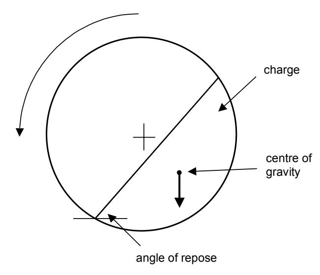
In the past many researchers have assumed that the charge takes up a shape and position as shown in Figure 2 that is largely invariant and which contains particles which move in a locked manner. Equations based on a torque-arm or a potential energy approach were then developed. It has been shown (Morrell, 1993) that both of these approaches yield identical equations, as does a third one, which considers friction forces. The problem with the resultant equations when they are based on a conceptual view of the charge as shown in Figure 2 is not that the physics applied is incorrect but that the conceptual view and assumptions about how the media move are inaccurate.
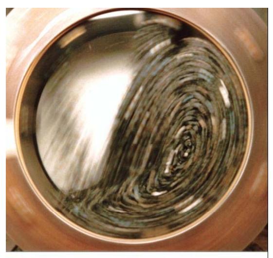
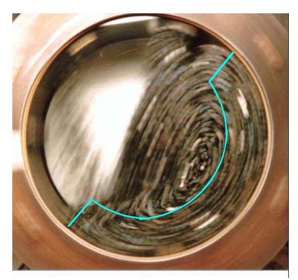
A different conceptual view has been taken by the author and is based on observations of the charge as it moved inside a glass-ended mill. A typical view is shown in Figure 3a. Figure 3b shows the simplification used by the author (outlined in pale blue) for the purposes of power draw modelling. This is based on the assertion that it is only the fraction of the charge that is not in freefall and not stationary that directly influences the power draw and that the crescent-shape shown in Figure 3b is a reasonable approximation of this material.
Using an energy balance approach, where power is taken to be the rate at which potential and kinetic energy is imparted to the charge, the following equation is obtained for a cylindrical vessel:
$$ P_{\text{net-cylinder}} = L\rho_c \int_{r_i}^{r_m} \int_{\theta_T}^{\theta_S} (V_r (rg \cos\theta + V_r^2)) d\theta dr $$ $$ (1) $$
where L = mill length
ρc = charge density r = radial position
rm = mill radius
ri = radial position of the charge inner surface
θ S = angular position of the shoulder and a principal function of the shell speed and charge volume
θ T = angular position of the toe and a principal function of the shell speed and charge volume
Vr = tangential velocity at radial position r and a principal function of the shell speed and charge volume
FACTORS INFLUENCING POWER DRAW
Equation 1 contains a number of variables, some of which are themselves complex functions of other variables. These are discussed below. Shell speed - this will affect the rate at which energy is imparted to the charge as well as the position of the toe and shoulder.
Mill filling - changes in filling will change the mass of charge which has to be moved by the mill. The position of the toe and shoulder will also vary.
Charge density - due to differences in density of different ores and the much higher density of steel balls, AG, SAG and ball mills will have different charge densities. The slurry density and how much of the voidage in the charge is occupied by slurry will also influence the charge density. To accurately determine the charge density the volume of rocks, balls and slurry must be know together with their densities. Also necessary is the voidage (also referred to as porosity) in the ball/rock charge as this dictates how much of the charge volume is occupied by slurry/air. In the literature it is often assumed that the voidage is 40% of the volume occupied by the charge. This is reasonable in a static charge but is questionable for a dynamic charge. Experiments conducted by Latchireddi (2001) showed that the dynamic voidage is much higher (typically in the range 45-55%) and is a strong function of charge volume and to a lesser extent shell speed (Figure 4).
Slurry level – this influences the charge density, which will increase as the slurry level increases. It also has a more direct impact on the power draw when the slurry level is such that it creates a slurry pool at the toe of the charge. Obvious cases where this occurs is in overflow ball mills. It may also occur in grate discharge mills where the flowrate of slurry is relatively high for the capacity of the discharge system. Schematically a mill which has a slurry pool (includes overflow ball mills) is shown in Figure 5 and is contrasted with a grate discharge mill in which a slurry pool has not formed. The effect of the slurry pool is to reduce power draw. This is intuitively seen in Figure 5 with reference to the grey-shaded section of the slurry pool. Due to its position on the "downward-rotating" side of the mill it helps rotation and therefore will reduce power draw. This behavior is responsible for the lower power draw seen in overflow ball mills when compared to grate mills of the same size, ball charge and speed.
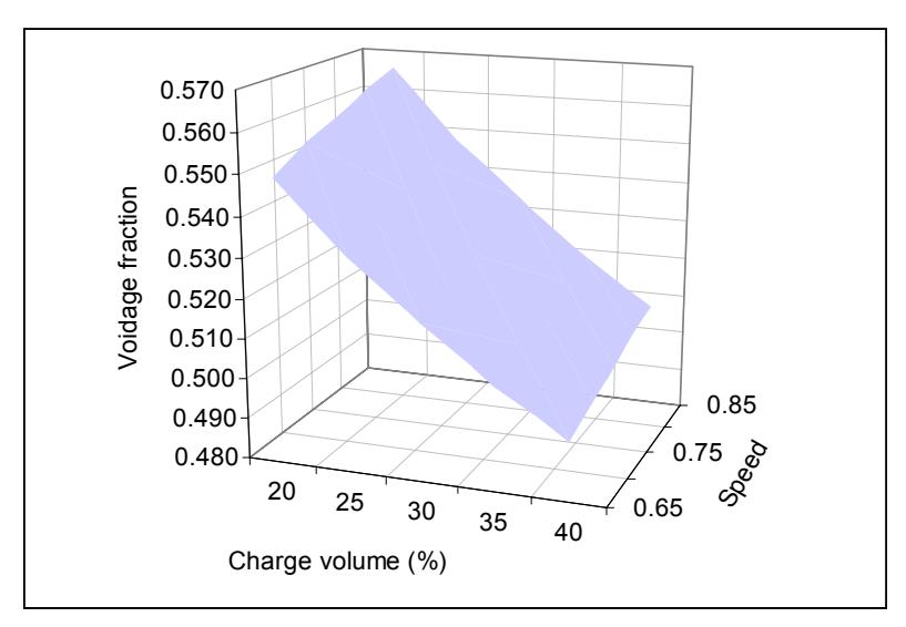
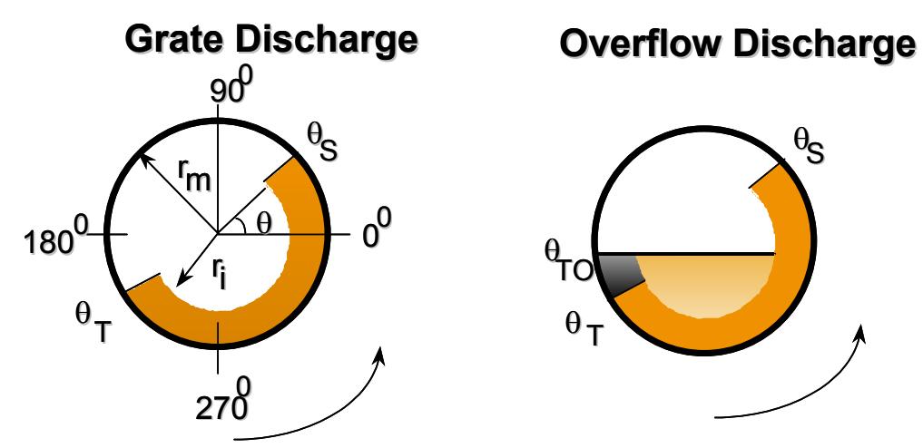
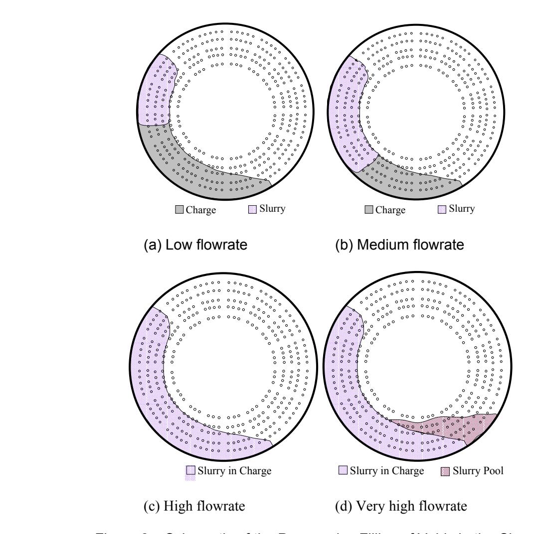
Figure 5 shows cases of no slurry pool and a well-established slurry pool condition. Where no slurry pool exists the voidage of the charge may only be partly occupied by slurry, this being dictated by the prevailing slurry flow rate. As the flowrate increases the slurry level and therefore the proportion of voidage occupied by slurry will increase. Experiments carried out by Latchireddi showed that a progressive occupation of voids in the charge occurs from the shoulder towards the toe. Eventually, when all of the voids are occupied slurry then accumulates at the toe as a pool. This is illustrated schematically in Figure 6. From a power draw viewpoint this result indicates that the charge density, as influenced by slurry, is not necessarily uniform throughout the charge. Equation 1 therefore cannot be applied to the charge en-masse but must be applied to the slurry portion of the charge independently. The power draw associated with the slurry can then be added to that for the rock/ball charge to give the total.
Cylindrical or conical end sections - a mill with conical ends will hold additional media and slurry, which will result in a higher power draw than a cylindrical mill with the same dimensions as the cylindrical section of the conical-ended mill. Equation 1 must therefore be modified so that the power associated with the charge in the cone ends can be predicted. The resultant equation is given below:
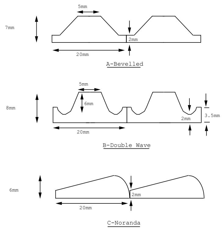
Lifter type - different lifter profiles/heights will change the amount of lift given to the charge in direct contact with the lifters. However, experiments with a glass-ended mill have shown that for the bulk of the charge that is not in direct contact with the lifters, differences in the amount of lift due to changes in lifter design are difficult to detect. Figure 7 shows a schematic of three designs that were tested in a 300mm laboratory mill (Morrell, 1993). Figure 8 shows how the lift, as measured by the angular displacement of the shoulder of the bulk of the charge, varied between lifter types as the speed was changed. Apart from at very high speeds the results as shown in Figure 9 indicated little difference. At high speed, however, there was a significant difference, the higher profile and more angular lifters (A and B) being found to fully centrifuge at a lower speed. This is supported by experience with variable speed industrial mills where it has been found that to operate at higher speeds the lifter face angle has to be reduced. Further evidence of this trend comes from high-speed mills in South Africa, which typically run with grid liners that have a very low profile.
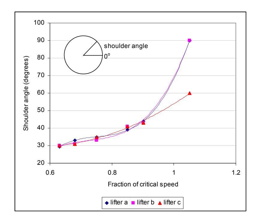
From a power modelling viewpoint the effect of lifters therefore need only be taken into account for the outermost layers of the charge. To do so with the conceptual view of the charge as shown in Figure 5 is relatively easy. The charge needs only to be divided into two contiguous crescent shapes each with its own relationship between shoulder/toe position and mill filling and speed. This structure is similar to that proposed by Moys (1990).
Mechanical/Electrical losses – industrial mill power is usually measured on the input side of the motor, whereas many pilot and laboratory scale mills are fitted with torque gauges, usually on the final drive shaft. The torque is then converted into power using the product of the torque and rotational rate of the shaft. Power in this case would not include any motor or reducer (gearbox) losses. To predict motor input power, therefore, and hence be in a position to compare the prediction with measured power from an industrial mill requires the addition of a term to account for electrical and mechanical losses. These losses are proportionately higher in smaller mills (in pilotscale mills they can account for up to 20% of the motor input power). In large diameter mills this proportion is much smaller (probably of the order of 6-8%). These losses are also a function of the type of drive train, the type of bearings and the general mechanical state of the mill. The problem from a modelling viewpoint is that there are no published data for industrial-scale mills relating to accurate measurements of the motor input power and that delivered to the shell. The nearest to it are measurements of the so-called no-load power which is drawn when the mill rotates when empty. Morrell (1996) used such data to estimate what the mechanical and electrical losses were with respect to changes in mill size.
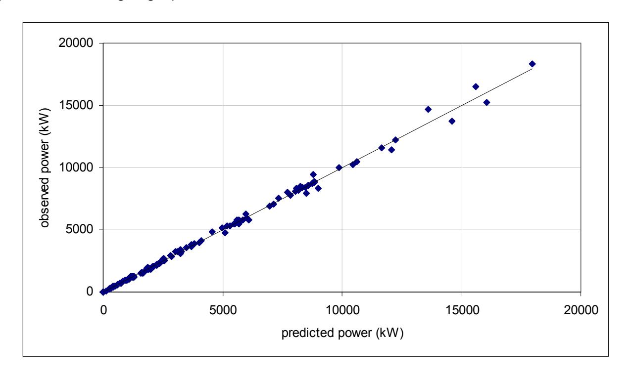
With all of the preceding factors correctly incorporated into a model it should be able to accurately predict mill power draw under most of the circumstances found in practice. Such appears to be the case from the plot given in Figure 10. This is a comparison of the predictions of the model with over 125 data sets. These cover ball, AG and SAG mills ranging in diameter from 2 ft to 40 ft and power draws from 6 kW to almost 20000 kW. The standard error associated with the predictions as 5% giving a precision of about +/- 10% at the 95% confidence level.
CONCLUSIONS
Using an appropriate conceptual view of the rotating charge inside tumbling mills and incorporating a description of the charge dynamics which relates the shape and motion of the charge to its composition and the speed of the shell it is possible to generate a model of the power draw which has a precision of +/- 10% at the 95% confidence level.
REFERENCES
Arbiter N. and Harris C.C., 1982. Scale-up and Dynamics of Large Grinding Mills - a Case Study. Design and Installation of Comminution Circuits, Mular A.L. and Jergensen II.G.V. (eds) AIME, New York, Ch 26, pp 491-505.
Austin L.G., 1990. A mill power equation for SAG mills. Minerals and Metallurgical Processing. pp 57 - 63.
Bond F.C., 1961. Crushing and grinding calculations. Allis Chalmers Publication No. 07R9235B, Revised Jan.
Bond F.C., 1962. Additions and revision to "Crushing and grinding calculations" (Bond, 1961).
Fuerstenau D.W., Kapur P.C. and Velamakani B., 1990. A multi-torque model for the effects of dispersants and slurry viscosity on ball milling. International Journal of Mineral Processing, Elsevier, Amsterdam, pp 81 - 98.
Harris C.C., Scknock E.M. and Arbiter N., 1985. Grinding mill power consumption. Mineral Processing and Technology Review, Vol 1, pp 297 - 345.
Hogg R. and Fuerstenau D.W., 1972. Power relationships for tumbling mills. Trans. SME/AIME, 252, pp 418 - 423.
Latchireddi, S.,
Liddell, K.S., 1986. The effect of mill speed, filling and pulp rheology on the dynamic behaviour of the load in a rotary grinding mill. M.Sc. Thesis, University of Witwatersrand, Johannesburg, South Africa.
Mishra B.K. and Rajamani R.K., 1990. Numerical simulation of charge motion in a ball mill. Preprints of the 7th European Symposium on Comminution, pp 555 - 563.
Morrell, S.,1993. The optimization of power draw in wet tumbling mills. Ph.D. Thesis. The University of Queensland, Australia, 1993
Morrell, S. 1996. Power draw of wet tumbling mills and its relationship to charge dynamics - Part 1: a continuum approach to mathematical modelling of mill power draw. Trans Inst Min Metall, Section C Vol 105, C43-53.
Morrell, S. 1996. Power draw of wet tumbling mills and its relationship to charge dynamics - Part 2: an empirical approach to modelling of mill power draw. Trans Inst Min Metall, Section C, Vol 105, C54-62.
Moys M.H., 1990. A model for mill power as affected by mill speed, load volume and liner design. Preprints of the 7th European Symposium on Comminution, pp 395 - 607.
Rose, H.E. and Evans D.E., 1956. The dynamics of the ball mill, part I: power requirements based on the ball and shell system. Proc. Inst. Mech. Engineers, pp 773 - 783.
Rose H.E. and Evans D.E., 1956. The dynamics of the ball mill, part II: the influence of the powder charge on power requirements. Proc. Inst. Mech. Engineers, pp 784 - 792.
White H.A., 1905. Theory of tube-mill action. Jour. Chem. Met. and Min. Soc. of South Africa, Vol V, pp 290.