LARGE DIAMETER SAG MILLS NEED LARGE DIAMETER BALL MILLS – WHAT ARE THE ISSUES?

S.Morrell

Principal Consultant

SMCC Pty Ltd, 26 Mermaid Place, Sinnamon Park, Qld 4073, Australia

ABSTRACT

The last five years have seen an increasing trend towards fewer comminution machines per grinding line with the result that units have increased considerably in capacity. Much attention has been paid to semi-autogenous and autogenous mills, which have now reached 12 m in diameter and draw 20 MW. Almost unnoticed has been a similar increase in ball mill size with units of 7 m being operated on at least 2 sites and 5 m plus units being commonplace. If the immediate "post-Bougainville Copper" literature are believed the present situation would have been considered unthinkable due to a belief by some that mills in excess of 5 m behaved in a different manner to smaller units. This paper reviews some of the issues related to sizing of large diameter ball mills including power draw, residence time, feed size and the applicability of Bond's equations. Data from a wide range of ball mills are used to indicate a "safe" operating envelope for large mills.

INTRODUCTION

The last five years have seen a continuing trend towards fewer comminution machines per grinding line with the result that units have increased considerably in capacity. Much attention has been paid to semi-autogenous and autogenous mills, which have now reached 12 m in diameter and draw 20 MW. Almost unnoticed has been a similar increase in ball mill size with units of 7 m being operated on at least 2 sites and 5 m plus units being commonplace. To determine whether there is any evidence that there are any trends in performance associated with diameter, operating data from a large range of ball mills were analysed. These data included power draw, flowrate and size reduction performance. Much of the data relate to ball mills treating ag/sag mill circuit products but some were from crushing-ball mill circuits. The data were analysed in a number of ways. The power draw data were compared to predictions using a power model, the size reduction data were compared to predictions using Bond's formulae and the flowrate data were used to estimate superficial velocities and residence times. In the following sections the results of each of these analyses is described.

POWER DRAW

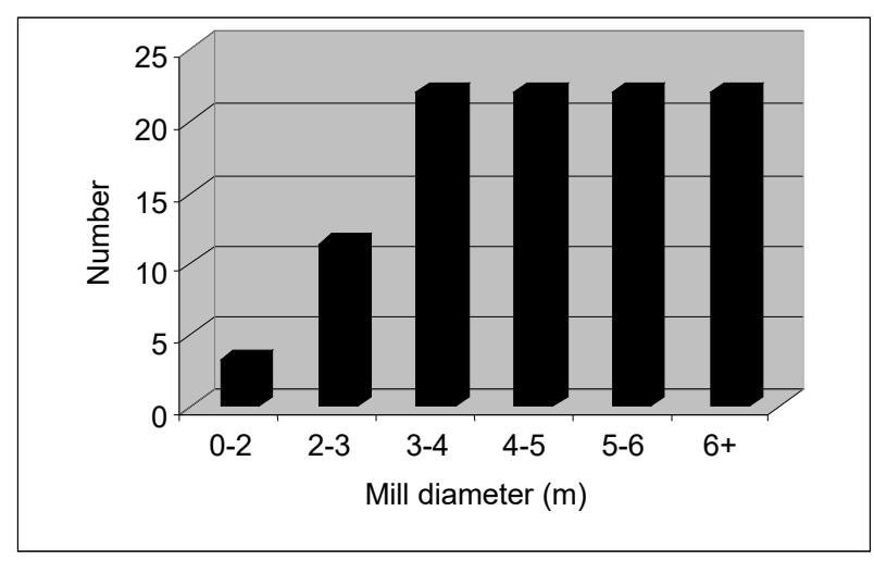
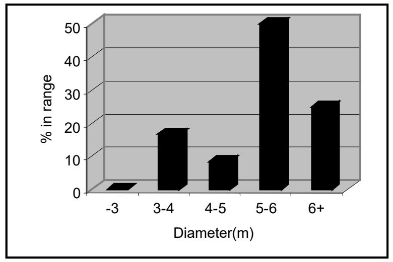
Morrell (1996) published a large database of ball, ag and sag mills. This data base has been extended considerably since then and includes data from ball mills up to 26ft in diameter drawing over 10 MW as well as sag mills up to 40 ft in diameter drawing 18 MW. Ball mill data sets number 59 and a histogram of the diameters of these mills is given in Figure 1. Since 1996 the author has made a number of modifications to his original model which now includes a dynamic porosity term, a slurry pool term for ag/sag mills operating in this manner as well as allowance for mills with wrap-around motors.

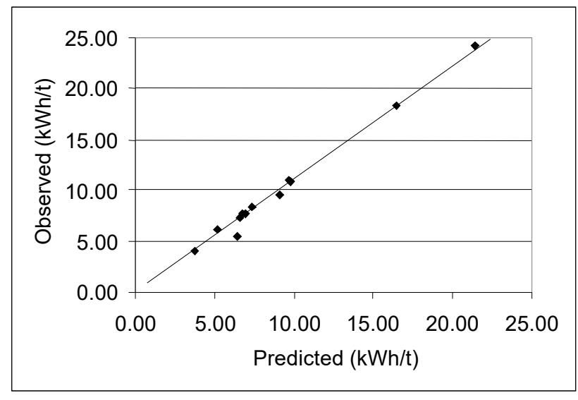
Applying this model to predict the power of ball mills gives the results shown in Figure 2. From an accuracy viewpoint it can be seen that the predicted values are highly correlated with the observed values. The mean relative error is 0.2% with an associated standard deviation of 4%. Hence the model should be accurate to within 0.2% with a precision of +/- 7% at the 90% confidence level.

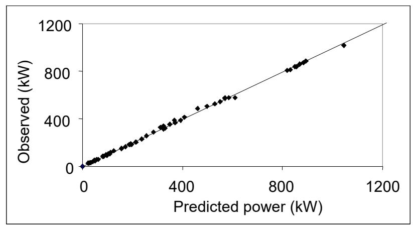
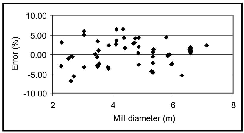
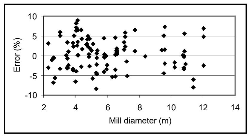
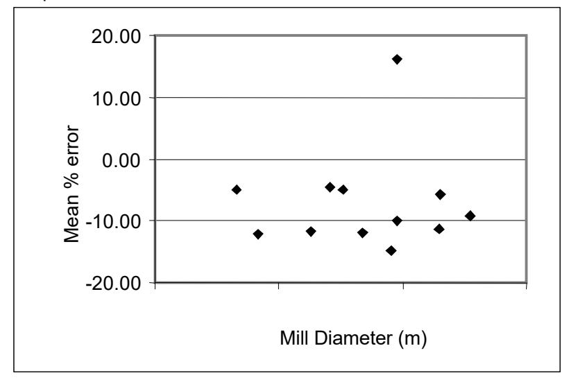
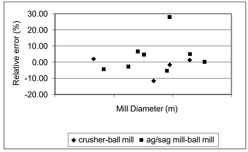
It should be noted that the model used to generate Figure 2 has an underlying diameter scaling exponent of 2.5. To further support the fact that this exponent is the correct one rather than 2.3 or 2.8 as claimed by some, the errors using the model were plotted against mill diameter. The results are given in Figure 3. It can be seen that the errors are randomly distributed ie there is no bias in the model with respect to mill diameter. This relationship is further backed up by including ag and sag mill data, which extend the diameter range to 12m. These results are shown in Figure 4. Once again the errors are seen to be randomly distributed.

It is interesting to review the results given in Figures 3 and 4 in the light of what Bond called a "slump" factor which accounted for what he claimed was a loss in power which was observed as mill diameter increased and if the ball size reduce below a certain level. This, he argued, was the result of excessive slippage between ball layers that became more pronounced as the number of layers increased. Bond modified his original slump correction in 1962 and Rowland subsequently revised it again (1972). Rowland stated that a loss in power would not occur in mills greater than 12 ft providing the ball size was greater than 1/80th of the mill diameter. If it were less than 1/80th the following empirically-derived power (S) should be subtracted per short ton of balls:

S = 0.15D – 0.5B

Where D = mill diameter inside liners (ft)

B = ball size (inch)

If a power loss was indeed occurring in the manner indicated above, then given a typical ball size of 65mm (2.5inch), such power loss would only be noticeable in mills with diameters greater than 80 x 65mm or 5.2 m. The error plot in Figure 3 shows no such trend. The data, therefore, do not tend to support the idea that power is lost due to ball slippage, at least with the balls used in the mills in the data base.

The previous arguments do not preclude the possibility that power losses may occur if the ball size is reduced too far for a given mill diameter, only that it is not noticeable as a pronounced effect in the data. Morrell (1993) in his PhD thesis described the ball size effect by calculating the slip between each ball layer. Using this model, results suggested that for an 8m ball mill running with 65mm balls, the power loss would only be 3%. Given the small magnitude of this effect therefore makes it unlikely that it would be discernible at the plant level given that power fluctuations can often be greater than +/- 5%.

SIZE REDUCTION PERFORMANCE

The most established technique for determining size reduction performance is by applying Bond's equations (Bond, 1961) or some adaptation of them such as described by Rowland (1972). Another way is via simulation where a model whose parameters are determined from the dimensions of the mill and operating conditions, predicts the product size distribution. Power draw is determined independently using the same mill dimensions and operating conditions. This contrasts with Bond's approach where the power requirement is determined directly from the feed and product size specifications with limited reference to the design of the mill and the operating conditions.

Bond's Technique

Bond's equation for the specific power requirement to reduce a feed with a specified F80 to a product with a specified P80 is given below.

$$ W = 10Wi (P^{-1/2} - F^{-1/2}) $$ (1)

Where: W = Specific motor output power (kWh/t)

Wi = Work index (kWh/t)

It is pointed out that Bond stated that this equation "conforms with the motor output power to an average overflow ball mill of 8ft interior diameter grinding wet in closed circuit" and should therefore give the required rated (nameplate) motor power. It is not motor input power, which is typically that which is recorded in operating plants and which also includes power losses due to motor inefficiency. It is also not the power at pinion, though it is often used as such even though it will include power losses due to bearing and pinion/ring gear inefficiencies but will not include motor and reducer (gear box) inefficiencies. How much each of these inefficiencies amounts to is a moot point and will depend on factors such as the type of bearing/lubrication system, drive system (eg conventional or gearless), motor, and whether the motor is operating at full power.

Equation 1 also does not account for classifier inefficiencies. Hence where Wi is determined from a Bond laboratory test it will implicitly indicate the specific power for a circuit using a perfect classifier.

Having developed equation 1 Bond proceeded to modify it with a range of "efficiency factors" which attempted to cater for the differences in feed and operating conditions that are found with different circuit designs and ore types. For ball mills these were:

EF1 - Dry grinding

EF2 - Open circuit ball milling

EF3 - Mill diameter

EF4 - Oversize feed

EF5 - Grinding finer than 70 microns

EF7 - Too small reduction ratio

For this study only the mill diameter (EF3 factor) and the oversize feed (EF4) factors were considered for this study.

The diameter factor was introduced by Bond due to what he stated was an increase in mill efficiency as the diameter increased above 8ft. However, his argument as to why this should be so is tenuous to say the least. The specific power using equation 1 is multiplied by EF3 where the mill diameter exceeds 8 ft.

EF3 = (8/D)0.2

Where D = mill diameter in feet

Rowland (1972) modified the application of EF3 and stated it should be used up to mills of 12ft then kept at the 12ft value for all larger mills. Why mills should increase in efficiency only between the diameters of 8 and 12 ft appears odd and no plausible reason has been provided why this should be so. The EF4 oversize feed factor was stated by Bond to cater for those cases where the feed size was coarser than a specific size limit (Fo), which was a function of ore hardness. Bond argued that if the feed ore was coarser than this, bigger balls would be needed to break the coarser feed particles at the expense of finer grinding of smaller particles. Conversely if smaller balls were used to grind the finer particles they would not break the coarser particles. Either way a grinding inefficiency would result. The EF4 factor is applied only when the F80 is greater than Fo (for which Bond gives a formula) and has a value greater than 1. The specific power is multiplied by EF4. Rowland (1975) modified the use of the EF4 equation and recommended that the rod mill work index should be used to calculate Fo in cases where the rod mill work index was greater than the ball mill work index. In 1978 Rowland further revised his recommendations and suggested that not only should Fo be calculated as above but that the rod mill work index should be used for calculating the specific energy from the new feed F80 to 2.1mm (only when the rod mill work index was greater than the ball mill work index). From 2.1mm to the final grind size the ball mill work index should be used as normal.

Oversize Feed

Unfortunately there are little published data on the accuracy of Bond's equations or the modifications to them that Rowland subsequently introduced. Blaskett (1969) provided some relevant data for relatively small mills and concluded that application of the efficiency factors produced poorer results than if they were not used at all! Unfortunately he published only one data set that required the use of the oversize feed factor. This clearly showed that for mills grinding to relatively coarse product sizes the EF4 equations in their original form are not appropriate and lead to gross over-estimates of power requirement. Rowland (1973) also published some data that are very valuable in that they do have several mills with coarse feeds. Rowland's analysis of these data concluded with this comment: "The work index comparisons….were not consistent without the application of this (EF4) factor". Rowland's data did not cover very coarse product sizes such as that reported by Blaskett, and all of his data fell in the P80 range 175-250 microns with an average P80 of 200 microns. It is concluded that at least in this size range it is valid to apply an oversize feed factor. When grinding to coarser product sizes application of the EF4 factor can lead to unrealistically high power estimates. For these conditions a modified form of the EF4 equation has to be applied.

Diameter Efficiency

The capacity problems experienced by Bougainville Copper (Steane and Hinckfuss, 1979) brought into review the efficiency of larger mills and the effect of coarser feeds. It is difficult after so many years to unravel the causes of the problem. However, the symptoms were clear – very high recirculating loads of coarse material and throughput lower than expected. At the time some placed blame on the size of the mill as it was the biggest diameter mill of its day (5.5m) and hence lead to the belief by some that mills with larger mill diameters were less efficient than smaller ones. Others, however, pointed out that a similar sized mill at Pinto Valley had no apparent problems and blamed the coarse feed to the Bougainville mill. Since then much larger mills have been built, treating a wide range of feeds, with no reported capacity problems. One well documented case of a successfully operating large mill with a relatively coarse feed was that installed at Sydvaranger (Forsund et al, 1988), which was a 6.5m diameter machine. This unit was operated in open circuit and was claimed to have a lower operating work index than smaller units at the same site. These results therefore appear to be in direct contrast to those claimed for Bougainville.

Evaluation of Bond's Equations for Larger Diameter Mills

To indicate whether mills with larger diameters behave differently and at the same time determine the validity of the Bond approach, data from 12 different mills was compiled. These data, which include feedrate, recycle load, power draw, feed and product sizing as well as Bond ball work indices were collected during circuit audits. In a number of circuits several repeat audits were conducted and the average values were used. A breakdown of the diameters of the mills is given in Figure 5.

Equation 1 was applied using the measured F80 and P80 values together with the laboratory work indices. As rod mill work indices were not available the oversize efficiency factor (EF4) was used as per Bond (1961). The diameter efficiency factor was applied as per Rowland (1972). The results were compared with the measured plant kWh/t for the ball mill circuits. As equation 1 relates to motor output and the plant data relate to motor input power the Bond results were divided by 0.97 to make them compatible (ie it was assumed that motor power losses were 3%). The results are given in Figure 6 and show good correlation, though in all cases but one the approach underestimates the true power requirement.

To determine whether any trend existed that was associated with mill diameter, the relative error was plotted against mill diameter as shown in Figure 7. Positive errors denote that the plant kWh/t was lower than predicted and hence operated better than expected. Overall the data in Figure 7 indicate that there is nothing to suggest that the larger diameter mills perform less efficiently than the smaller ones.

Interestingly with the ag/sag circuits, application of the so-called phantom cyclone, where the ag/sag mill product size and flowrate are modified prior to applying Bond's equations, did not improve the overall prediction. However, by appropriate modification of the EF4 equation and setting EF3 to unity, the results given in Figure 8 were obtained. All but one of the results falls within a band of +/- 10%.

The 2 data points in Figure 8 which indicate the most error are those of Bougainville Copper and a circuit which is severely ball mill power limited and which is run with exceedingly high recycle loads (500+%).

What Is the True Performance of a Circuit?

Even ignoring the 2 extreme points mentioned in the previous section still leaves a fair degree of scatter in the remaining data. This scatter is the result of a combination of inherent errors in the Bond equations plus experimental errors associated with obtaining circuit performance data, conducting the Bond laboratory test and the representativeness of the sample used in the test.

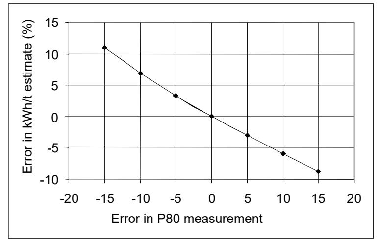
Particularly with large diameter mills, where flowrates are often very high, accurate sampling of streams for auditing purposes becomes very difficult. This has important implications with respect to evaluating what is the true performance of the circuit. To illustrate this point Figure 9 shows how much 5 micron incremental errors in measuring the final product p80 make to the apparent operating work index . The true P80 in this case is 100 microns, but only a 5 micron error in its measurement causes almost 5% error in the apparent operating work index. Repeat audits of circuits reflect this affect and it is not uncommon for variations of +/ 20% in the apparent work index of a circuit under conditions which are nominally identical.

TRANSPORT AND MIXING

The analysis of the Bougainville Copper circuit lead to a number of hypotheses regarding its poor performance. One of these was associated with poor mixing and high flowrates (Harris and Arbiter, 1982) that resulted from its large diameter. Arbiter and Harris suggested that in the Bougainville case high flowrates lead to low residence times that caused high circulating loads. For a given ore, as the mill diameter increases power draw and hence throughput will typically increase in the ratio D2.5. Flow cross-sectional area only increases as D ² and hence the velocity of slurry passing through the mill will increase and its residence time will decrease as the mill diameter increases. However, the energy imparted to the slurry during its passage through the mill will also increase. Rowland (1988) provided a similar view and suggested that in larger diameter mills residence time was important as well as ensuring slurry velocity was not so great that it disrupted grinding action. It is therefore instructive to look at a range of operational mills and see whether the data indicate whether the Bougainville mill suffered from these problems and whether they were diameter related.

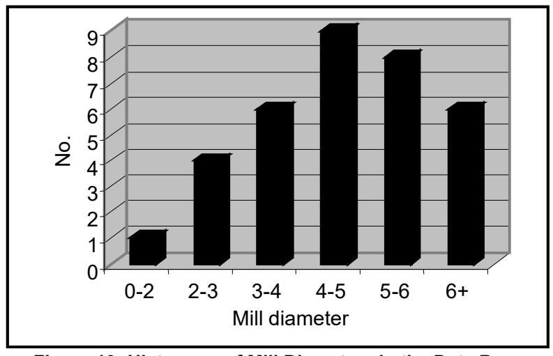
A total of 34 mills were examined, the majority being relatively large diameter units. Figure 10 gives details of the range of diameters of these mills.

Superficial Velocity

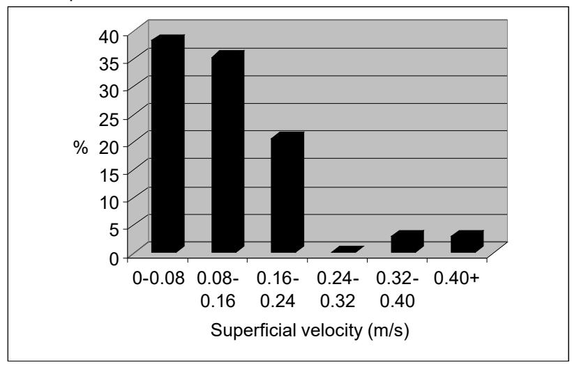
For each of the mills a superficial velocity was calculated based on the estimated cross-sectional area of the slurry pool. This was on the assumption that the slurry pool extended from the toe of the dynamic ball charge to the discharge trunnion. These calculations used a simplified picture of the slurry pool and were intended only to ensure that the size of the slurry pool was related to the ball charge in a systematic manner. This was considered to be important as the experience at Sydvaranger (1988) was that by dropping the ball load from 40% to 22% coarse particles in the mill discharge were drastically reduced (the amount of finer grinding also reduced considerably). This was attributed to the classifying effect of the very large slurry pool in the 22% load case. The low superficial velocity in the pool would allow coarser particles to settle-out and hence stay in the mill longer. A superficial velocity based simply on mill diameter would not indicate any difference between the ball load conditions whereas one based on ball charge voidage would incorrectly give a higher value for the low ball charge scenario. Superficial velocities based on the slurry pool are therefore considered to be more valid in this context. A histogram of the superficial velocities is shown in Figure 11. For comparison purposes the superficial velocities in a 1m pilot mill are of the order 0.001-0.01 m/s.

Figure 11 shows a bimodal distribution with the majority of mills falling in the 0-0.24 m/s range. A small proportion fall in the +0.32 m/s range. This group contains 2 mills, one of which is Bougainville Copper. The second mill is grossly overloaded and suffers from problems of steel ball ejection. From this analysis it would therefore appear that if superficial velocities reach levels over 0.32 m/s then capacity problems may result with associated coarse particle and/or ball ejection. For velocities less than 0.24 m/s no reported problems would appear to exist. In the range 0.24-0.32 m/s there are no data but velocities falling in this range should provide a warning of potential problems. These data also suggest that pilot mill results may be somewhat optimistic in terms of treatment of coarser particles.

Mean Residence Time

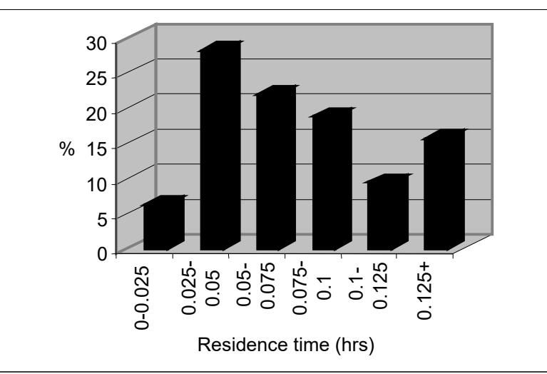
The mean residence times for each mill were also calculated using a slurry volume comprising the estimated slurry pool plus the slurry in the ball charge interstices. A histogram of the results is shown in Figure 12. Once again Bougainville is at the extreme end of the spectrum in the 0 – 0.025 hour (1.5mins) category. Residence times in this category would therefore indicate possible grinding problems.

CONCLUSIONS

On the basis of data collected from circuit audits of a wide range of large diameter mills the following conclusions are drawn:

• · The power draws of large diameter mills follow the same relationships that hold for smaller diameter mills as described in Morrell's model.
• · Bond's equations for determining ball mill specific power requirements produce results which are well correlated with observed values, although they are somewhat offset.
• · Appropriate adjustment to Bond's equations, including setting the diameter efficiency factor to unity and modifying the oversize feed efficiency factor, removes this offset and indicates that the specific energy of the majority of mills can be predicted to within +/- 10%.
• · No indications were found that the accuracy of Bond's equations was related to mill diameter.
• · The equations appear to be equally valid for ball mills following ag/sag mills and crushers.
• · The use of the so-called "phantom cyclone" approach where the ag/sag mill discharge is corrected prior to application of Bond's equation did not improve overall accuracy.
• · Analysis of residence times and superficial velocities pointed to the existence of a relatively safe operating envelope outside of which coarse particle ejection and high recycle loads are likely to result.

· These parameters can be calculated at the design stage to determine whether a specified mill is likely to fall outside of this envelope

REFERENCES

BLASKETT K.S., 1969. Estimation of the Power Consumption in Grinding Mills. Proceeding of the Ninth Commonwealth Min. Metall ., 3, pp 631-649.

BOND F.C. 1961 (revised 1962). Crushing and Grinding Calculations. Allis-Chalmers publication O7R9235B

FORSUND B., NORKYN I., SANKVIK K.L. AND WINTHER K., 1988. Sydvarangers 6.5m diameter x 9.65m ball mill. XVI Int. Mineral Proc. Congress (Ed. Forssberg E), pp171-183

HARRIS C.C. AND ARBITER N. 1982. Grinding Mill Scale-up Problems. Mining Engineering . January,pp 43-46

MORRELL S., 1996. Power Draw of Wet Tumbling Mills Parts 1 and 2. Trans. Inst Min. and Metall . (section C), Vol 105.

MORRELL S., 1993. Power Draw of Wet Tumbling Mills . PhD thesis, Uni. Of Qld., Australia.

ROWLAND C.A. Jnr. 1972., Grinding Calculations Related to the Application of Large Rod and Ball Mills. Allis-Chalmers Publication 22P4704.

ROWLAND C.A. Jnr. 1973., "Comparison of work indices calculated from operating data with those from laboratory test data". Proc. 10th IMPC , pp 47-61

ROWLAND C.A.JNR AND KJOSS D.M. 1978 (revised 1980). Rod and Ball Mills. Mineral Processing Plant Design . Mular and Bhappu (editors), SME, Chapter 12, pp 239-278.

ROWLAND C.A. Jnr. 1975., The Tools of Power Power: How to Evaluate Grinding Mill Performance Using the Bond Work Index to Measure Grinding Efficiency. Proc. AIME Annual Mtg, Arizona, USA.

ROWLAND C.A. 1988. Diameter Factors Affecting Ball Mill Scale-up. Int. Journal of Mineral Processing, 22, pp 95-104

STEANE R.A. AND HINCKFUSS D.A., 1979. Selection and Performance of Large Diameter Ball Mills at Bougainville Copper Ltd. Papua new Guinea. Proc. 11th C/wealth Min. and Met. Congress , Hong Kong, pp 577-584.