MAPPING OREBODY HARDNESS VARIABILITY FOR AG/SAG/CRUSHING AND HPGR CIRCUITS

S. Morrell

SMC Testing Pty Ltd 220 Tinarra Crescent Brisbane, Australia

ABSTRACT

Arguably the SMC Test® has become the most popular laboratory hardness test in the world with over 17,000 tests having been completed to date, covering over 650 different ore bodies. It is now routinely used in design, optimisation and orebody profiling projects. The test is unique in that from relatively small amounts of drill core it simultaneously provides parameters that are used in simulation modelling of AG/SAG and crushing circuits as well as work indices that are used in power-based equations for predicting the specific energies of AG/SAG/Crushing and HPGR circuits. The very large data base that has been accumulated has provided the opportunity to study the differences in variability from deposit to deposit. This paper describes and discusses the trends that have become apparent from the study of this data base. Recommendations for appropriate selection of sample numbers are also made which are based on these trends.

KEYWORDS

geometallurgy, SMC Test®

INTRODUCTION

The last 10 years has seen an increasing awareness of the need for detailed ore characterization data with which to map orebody hardness, regardless of the nature of the project. In the case of new project development the need to understand the breakage characteristics of the orebody is paramount if the comminution circuit is to be sized correctly for the duration of the life-of-mine. The need is no less different in optimisation projects where it is required to get the very best from existing comminution circuits. However, these requirements, in both new development and optimisation projects, are often at odds with budgets, particularly when the global financial situation is less favourable. However, this does not necessarily mean that accuracy should suffer, only that the ore characterisation testwork programme has to be more focused and streamlined. The following paper discusses a number of factors and guidelines that should be considered when faced with developing such programmes.

NECESSARY ATTRIBUTES OF A TESTWORK PROGRAMME

From a comminution perspective, an effective model, whether used for design or for geometallurgical purposes should be able to accurately predict the throughput of the comminution circuit from information concerning the breakage characteristics of ores that are planned to be delivered to the processing plant. To do so there are at least five important requirements. These are that:

• x sufficient and relevant samples have been identified, extracted and tested
• x appropriate ore characterisation tests have been chosen to describe the comminution properties of the orebody;
• x the model(s)/equations chosen to describe the comminution equipment in the circuit respond realistically to the values obtained from the chosen ore characterisation tests;
• x all of the above are integrated into an overall description of the operational response of the grinding circuit that also takes into account non-ore related influences e.g., equipment size, speed, ball load tc.
• x the final model/equations can convincingly demonstrate their accuracy through validation using real plant data.

WHICH LABORATORY TEST(S)?

Clearly, the laboratory test(s) that are chosen need to be compatible with the modelling approaches subsequently used at the design stage or development of the geometallurgical model, e.g., if the "variable rates" AG/SAG mill model in JKSimMet is to be used (Morrell and Morrison,1996) the laboratory test has to generate an A and b value, or if a Bond equation is utilised the appropriate Bond work index tests have to be carried out. Apart from this criterion, the metallurgist should also be aware of whatever inaccuracies are inherent in the laboratory tests that have been chosen.

One such test is the SMC Test®which arguably has become one of the most popular laboratory tests for orebody mapping, whether for design or geometallurgical modelling purposes. Since its availability in 2003, over 17000 tests have been conducted to date covering over 650 different ore bodies. Its popularity is due to a number of factors:

• x its requirement for relatively small amounts of sample, making it ideally suited for use with small diameter drill core,
• x its versatility in that it provides a range of parameters from the one test, including the JK A,b and ta values, the rock strength parameter, DWi, plus the associated work indices Mia, Mih and Mic which enable power-based calculations to be made of the specific energy requirements of grinding mills, High Pressure Grinding Rolls (HPGR) and conventional crushers respectively
• x its availability most metallurgical laboratories around the world are licensed to do the tests.

WHICH MODELS/EQUATIONS?

The choice of which models or equations to be used should be driven by their demonstrable ability to predict the performance of existing plants. The "more - the better" rule applies in that the more (and varied) data that exist to prove the accuracy of the technique, the stronger is the argument to adopt it.

In design studies the most relevant data with which to evaluate the suitability of a technique should be those from existing comminution circuits whose performance has been predicted then checked against high quality operating data from the same circuit. Regardless of claims by the developers of particular design/geometallurgical models/techniques about how suitable and accurate they are, if a large volume of appropriately varied data cannot be presented to validate claimed accuracy, metallurgists should be extremely wary of utilising such models/techniques.

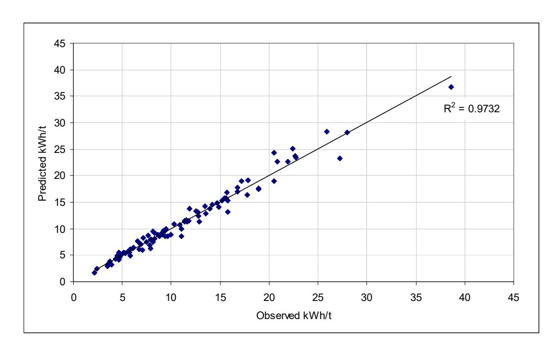
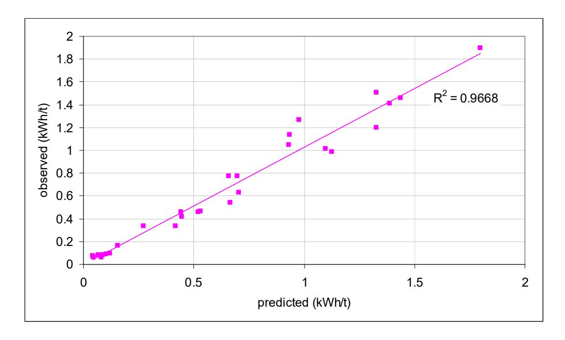
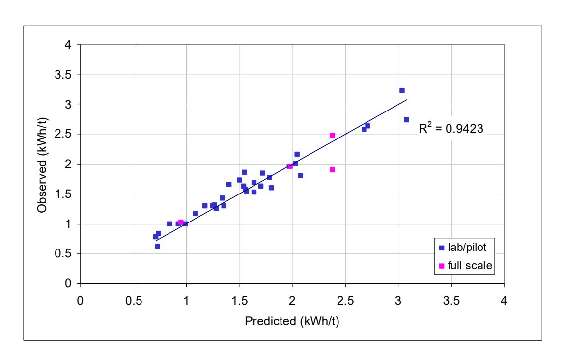
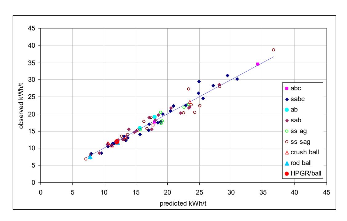
The development of the SMC Test® and the use of the parameters that it generates in predicting comminution circuit equipment and circuit performance has been well publicised (Morrell, 2004, 2008, 2009, 2010). The most recent development extended its use to predict both conventional crusher and HPGR performance (Morrell, 2009), its original development being for just AG and SAG mills. In the course of these developments the validity of the parameters and associated equations were assessed using large data bases of existing comminution circuits. The results from this assessment are demonstrated in Figures 1-4. Figures 1-3 illustrate how the SMC Test® work indices Mia, Mic and Mih are able to predict the specific energies of AG/SAG mills, conventional crushers (primary, secondary and tertiary) and HPGR circuits respectively. Finally in Figure 4 their accuracy when combined to predict the total comminution energy of different circuits is demonstrated. In cases where the circuits contained ball mills an additional parameter (Mib) was used which is obtained from a standard Bond ball mill work index test (Morrell, 2009).

HARDNESS VARIABILITY

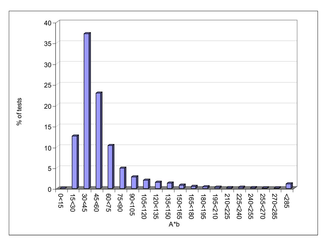
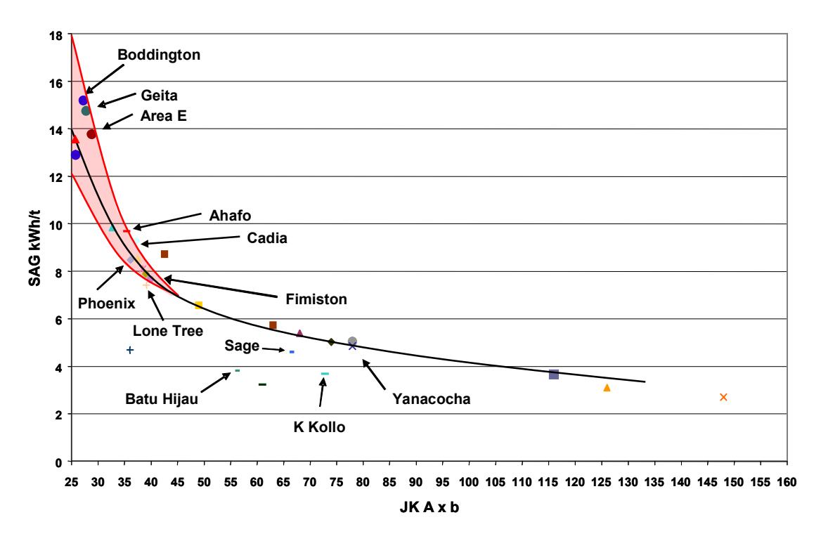
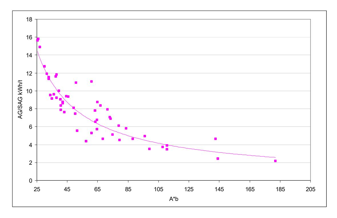
Due to the large number of SMC Tests® that have been carried out (17000+), the very broad spectrum of deposits that have SMC Test® data associated with them and the wide range of comminution attributes that can be described by the SMC Test®, accurate descriptions of orebody variability can be made. Figure 5 is once such example and shows a histogram of A*b values. Although A and b are principally used in the JK SAG mill simulation model, the product A*b has become popular in a qualitative manner to indicate hardness. However, it must be remembered that lower values of A*b indicate harder rock and is contrary to all other hardness parameters which increase with increasing rock hardness. As can be seen, Figure 5shows a highly skewed distribution which is due to the inverse relationship that A*b has with hardness. This relationship is apparent from the data in Figures 6 (Veillette and Parker, 2005) and Figure 7. They contrast with the linear relationship that is found with the DWi (Figure 8). The data in Figures 7 and 8 come from the same AG/SAG circuits in SMCC Pty Ltd's data base. It should be noted that they represent only the high aspect ratio mills in this data base. The trend for low aspect ratio mills is different, as aspect ratio has a significant impact on mill specific energy. The scatter in the data in both figures is largely due to differences in feed size, whether the circuits have pebble crushers, ball load and mill speed, all of which influence specific energy.

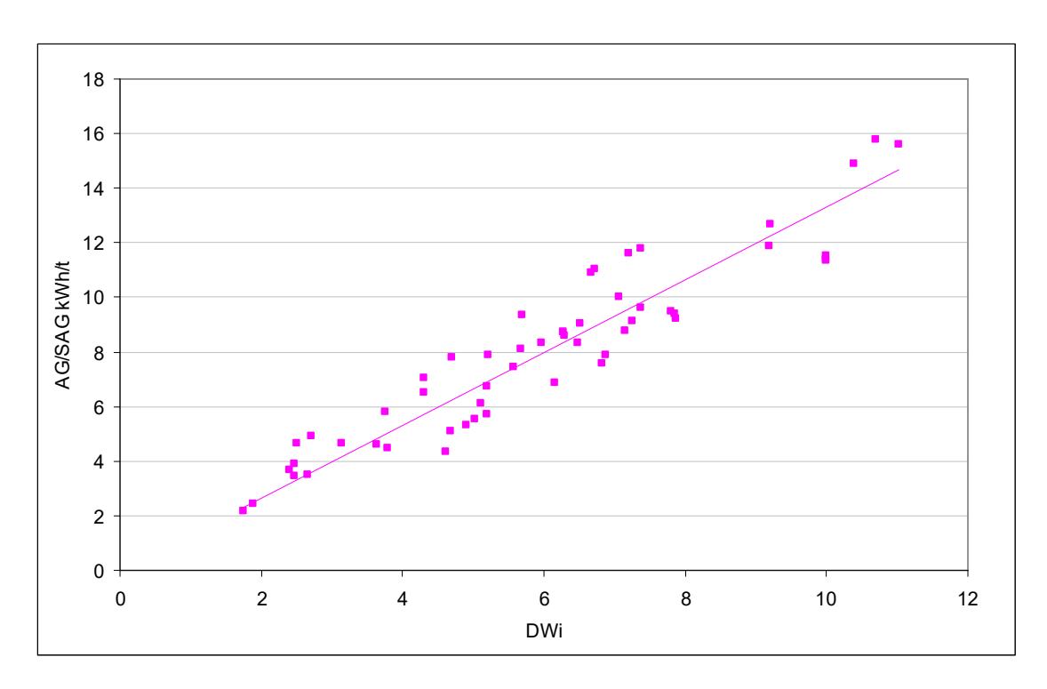
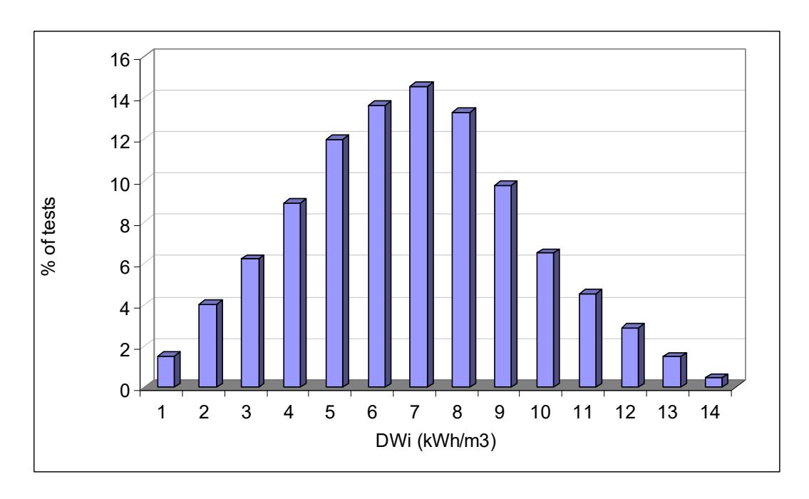
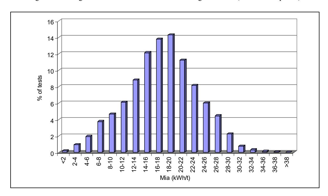
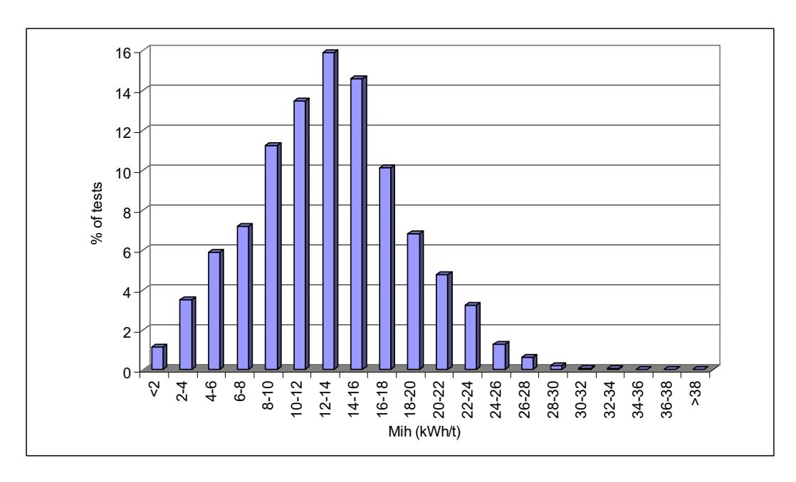
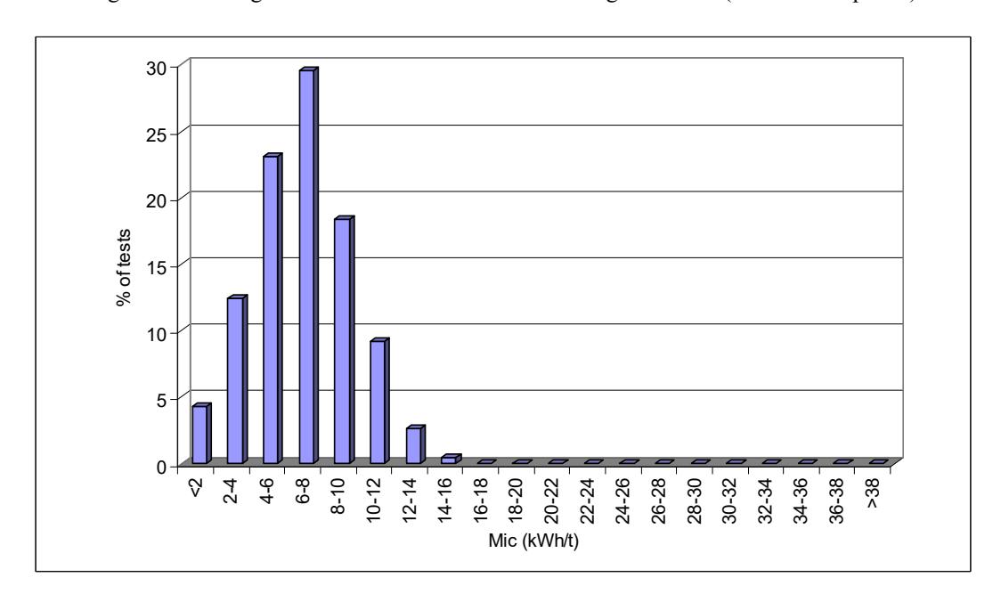
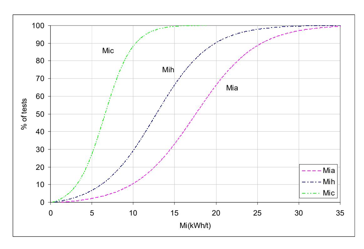
The linear relationship between the DWi parameter and AG/SAG mill specific energy results in a more normal looking distribution when the SMC Test® data base values are plotted in histogram form (Figure 9). This is also the case with the associated Mia, Mih and Mic values which are plotted in Figures 10-12. It is worth noting that although they all show normal-type distributions they have different mean/median/modes which is illustrated in the cumulative distributions shown in Figure 13. This figure indicates that Mia values are higher than Mih values which in turn are higher than Mic values. The Mi values are effectively work indices and are used with much the same equations to predict specific energy of tumbling mills HPGRs and conventional crushers (Morrell, 2010). Combined with their calibration with large data bases of existing circuits (Figures 1-4), their relative magnitudes reflect inherent difference in the energy efficiency of the associated comminution machines i.e., tumbling mills, HPGRs and conventional crushers. This puts conventional crushers ahead of HPGRs, which in turn have better energy efficiency than tumbling mills. This result confirms the original research of Schonert (1988, 1991).

HOW MANY SAMPLES?

There is no easy answer to this question though it is true to say "the more – the better". If the deposit is highly variable the required number of samples will be higher. Also the end use will also drive the number of samples required. Hence if samples are required for a pre-feasibility study the number will be relatively low, whilst if samples are required for a bankable study the numbers will need to be correspondingly higher. For the development of a geometallurgical model that has the ability to accurately forecast daily grinding circuit throughput, the number required will be at least an order of magnitude higher. In all cases a staged approach to sample selection and laboratory testwork is recommended to ensure that costs are kept to a minimum. Each stage should be designed to build on the knowledge gained from preceding ones, particularly concerning variability, both spatially within the pit as well as in terms of absolute hardness values.

The pre-feasibility study level is often the best opportunity to start accumulating useful information of the comminution properties of the orebody. At this stage little or no information is likely to exist on the comminution properties of the orebody and hence the metallurgist is faced with the decision of how many samples should be treated for this very first investigation. A good starting point is to use the distribution shown in Figure 14. This comes from SMC Testing's data base of over 650 different ore deposits. The figure shows the coefficient of variation (standard deviation/mean expressed as a percentage) of the measured DWi values from each deposit. The distribution is bi-modal, modal values being in the 15-20% and 35-40% classes, the average being 26%. Unfortunately the data base does not contain information other than SMC Test® values and the author is not in a position to determine whether this bi-modality can be traced back to geological descriptions of the nature and genesis of the orebodies. However, it is tempting to hypothesize that there is a very good physical reason why the distribution should have such a bi-modal shape.

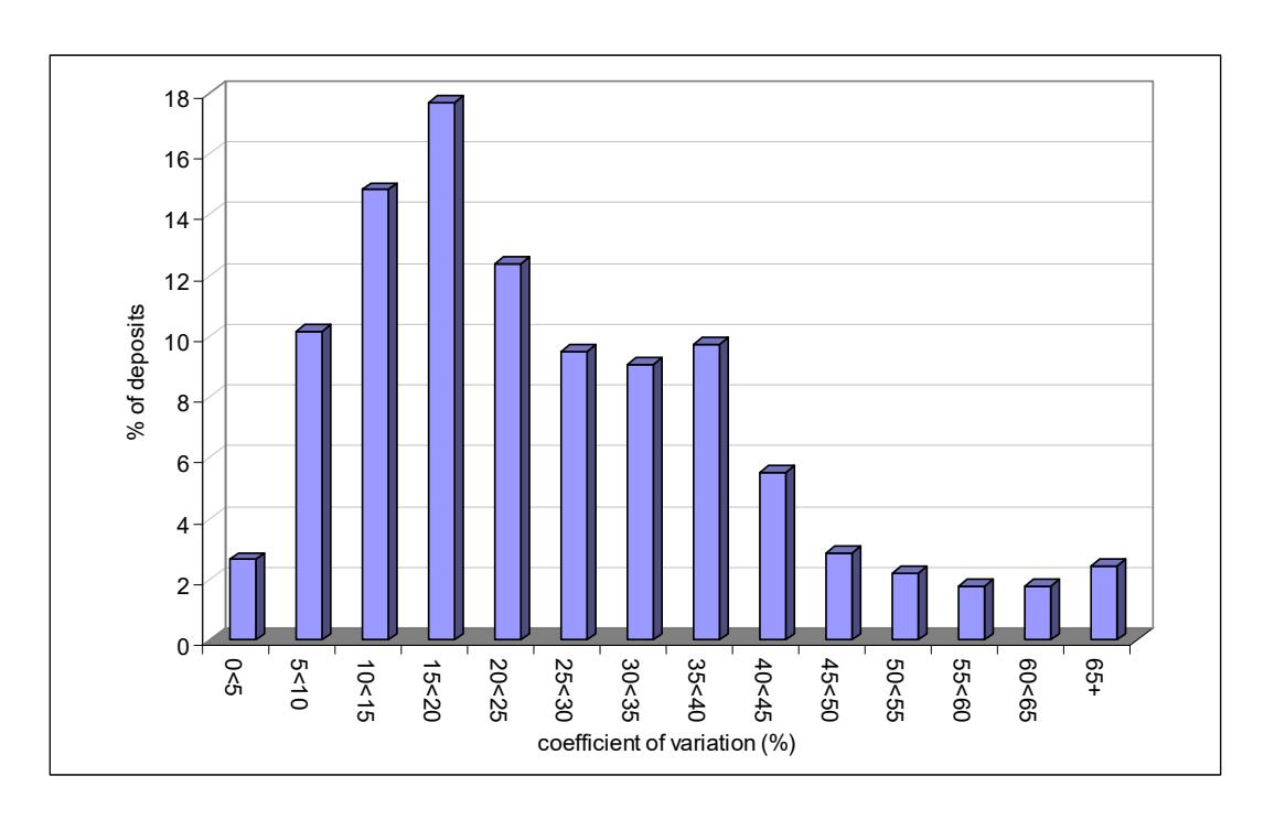
The data in Figure 14 can provide the basis of some simple calculations that can be used to guide the metallurgist's choice of how many samples should be taken and analysed in the first step of investigatingan orebody. Using classical statistics and assuming that the orebody has a variability of 15- 25% (ie the lower of the modal values), then choosing a total of say 10 samples should provide a mean hardness value for the deposit with a precision of 10% at the 90% confidence level. However if the variability is in the 35-40% class, to obtain the same level of precision the requisite number increases to 40. The minimum number of samples is therefore recommended to be 10. Note that these should not be composited samples but individual, discrete drill core intervals. The analysis of the data from these samples will provide an indication of the variability and can then be used to estimate how many more samples (if any) need to be treated to satisfy the accuracy for the pre-feasibility stage. If the indicated variability is say 35-40% then an additional 30 samples will be required. It is pointed out that these guidelines assume that the samples that are selected are representative of the orebody and that the resultant mean values can only provide global information. As the design stages progress through to a final bankable study, more definition is required to enable forecasts to be made of ore properties and hence throughput during at least the first few years of production. This requires further ore characterization. However, the results from the initial stage of testing should provide a firm basis on which to choose both the location of samples and numbers for further stages.

CONCLUSIONS

The choice of appropriate test(s) for orebody mapping should be made on the basis of its relevance to the associated comminution circuit and demonstrated accuracy of the techniques/equations that subsequently use the test results to predict plant performance.

This accuracy can only be truly demonstrated from analyzing large varied data bases of relevant plant performances. Regardless of claims by the developers of particular design/geometallurgical models/techniques about how suitable and accurate they are, if such data cannot be presented to validate claimed accuracy, metallurgists should be extremely wary of utilising such models/techniques.

In terms of the required number of tests, a staged approach is recommended in which, as projects develop from the pre-feasibility stage, knowledge of the variability of the deposit is progressively built and used to drive the number of tests required in subsequent stages.

Using classical statistics from variability data from over 650 deposits, guidelines have been developed which should help indicate the number of samples that are required in the initial stages of investigating the ore hardness of orebodies.

REFERENCES

Morrell, S.(2008).A method for predicting the specific energy requirement of comminution circuits and assessing their energy utilisation efficiency , Minerals Engineering, Volume 21, Issue 3, February, pp224- 233

Morrell, S.(2004). Predicting the Specific Energy of Autogenous and Semi-autogenous Mills from Small Diameter Drill Core Samples. Minerals Engineering, Volume 17, Issue 3, March, pp447-451

Morrell, S.(2009).Predicting the overall specific energy requirement of crushing, high pressure grinding roll and tumbling mill circuits, Minerals Engineering, Volume 22, Issue 6, May, pp544-549

Morrell, S.(2010). Predicting the specific energy required for size reduction of relatively coarse feeds in conventional crushers and high pressure grinding rolls, minerals engineering Volume 23, Issue 2, January, pp151-153

Morrell, S. and Morrison, R. (1996). AG and SAG mill circuit selection and design by simulation. Proc SAG '96, Vancouver, pp 769-790,

Schönert, K.(1988). A first survey of grinding with high-compression roller mills. International Journal of Mineral Processing., 22: pp401-412

Schönert, K.(1991). Advances in comminution fundamental, and impacts on technology, XVII International Mineral Processing Congress, Dresden, Sept 23-28 1991, Volume 1, pp 1-21.

Veillette, G., Parker, B.(2005). Boddington Expansion Project Comminution Circuit Features and Testwork, Randol Gold Forum Proceedings.