Modelling Approaches and Their Application in Comminution Circuit Design

S.Morrell

Managing Director, SMC Testing Pty Ltd, Brisbane, Australia, This email address is being protected from spambots. You need JavaScript enabled to view it.

ABSTRACT

Even 30 years ago pilot testing would still have most often played the leading role in comminution circuit design, even though mathematical models that describe comminution machine behaviour date back to the 1800's. Nowadays piloting is quite rare, instead modelling in its various forms is relied on in the choice and sizing of most new comminution circuits. This paper traces the history of comminution circuit modelling and describes a number of modelling approaches that are currently available to the comminution circuit designer such as so-called power-based and simulation modelling. The pros and cons of each are discussed as well as the accuracy that can be expected from their use in sizing comminution equipment using data that compare their predictions with values that have been measured from full scale operating plants.

INTRODUCTION

Neumaier (2004) describes mathematical modelling as " The art of translating problems from an application area into tractable mathematical formulations whose theoretical and numerical analysis provides insight, answers, and guidance useful for the originating application " whilst Verschaffel et al (2002) describe it as a " Cyclic process in which real-life problems are translated into mathematical language, solved within a symbolic system, and the solutions tested back within the real-life system ". There are at least four aspects from these definitions that are of particular relevance to this paper. The first is that any mathematical formulation can be considered a model (complex or simple), its only prerequisite being (the second aspect) that it provides useful (accurate) answers and that, thirdly, its accuracy is gauged by comparing its predictions with measured data from the system that it was designed to mimic and fourthly the model is modified where necessary until its accuracy is optimised. In the following sections a number of comminution models are described that have varying degrees of mathematical complexity. The extent to which they accurately predict full-scale plant data is reviewed.

POWER-BASED MODELLING

Model Equations

So-called power-based models are used to predict the specific energy of a comminution machine and/or comminution circuit. Given that are required to predict a single parameter, they tend to be the simplest of mathematical models and by far the most popular. Inherent to all of them is the representation of size distributions as single points eg 80th percent passing size. Underlying the adoption of this approach is the assumption that all size distributions have the same shape ie that they are linear and parallel in log-log space and that they all have approximately the same gradient.

One of the most popular and enduring power-based models was formulated by Bond (1952) and was based on what he called his "Third Theory". Bond went on to describe how his model could be used in practical design applications (Bond, 1961). His model is of the general form shown in equation 1.

$$ E = C(P_{80}^{-0.5} - F_{80}^{-0.5}) $$ (1)

Where:

E = net energy required per unit weight (specific energy)

\( P_{80} \) = \( 80^{th} \) percent passing size of the product \( F_{80} \) = \( 80^{th} \) percent passing size of the feed C = constant related to material properties

Bond developed laboratory ore characterisation tests for crushing, rod milling and ball milling such that so-called work indices ( \( W_{ic} \) for crushing, \( W_{ir} \) for rod milling and \( W_{ib} \) for ball milling) could be determined experimentally and used in equation 1 as follows:

$$ E = 10 W_i (P_{80}^{-0.5} - F_{80}^{-0.5}) $$ (2)

As pointed out by Hukki (1961) equation 1 is one form of the general differential equation proposed by Walker et. al. (1937) which can be written as:

where:

\( x = index describing the size distribution, eg <math>P_{80} \) , \( F_{80} \) n = exponent indicating the order of the process

If the exponent (n) in equation 3 is set to 1.5 and then integrated, Bond's equation results. Whilst if n=2 is used the equation proposed by von Rittinger (1867) is obtained (eq 4) and if n=1 is used Kick's (1885) equation is derived (eq 5).

$$ E = C(P_{80}^{-1} - F_{80}^{-1}) $$ (4)

$$ E = C (ln (F_{80}) - ln (P_{80})) $$ (5)

In all of these cases the exponent (n) is assumed to be constant for all conditions. However, both Charles (1957) and Holmes (1957) developed equations with a similar form (eq. 6) but with n being a variable which depended upon material type and the particular stress conditions that applied.

$$ E = C(P_{80}^{r} - F_{80}^{r}) $$ (6)

Where r varies with material type and stress conditions.

Hukki also concluded that the exponent was not constant but proposed it varied with the fineness of the size distribution. He therefore suggested that a more appropriate form of Walker et al's general differential equation was:

Despite the conclusions of authors such as Charles, Holmes and Hukki concerning the limitations of a fixed-value exponent, Bond's equation (2) has become one of two (see Morrell's equation 8 for the second one) recognised industry standards for predicting the comminution energy required to reduce rock from one size to another (Global Mining Guidelines Group, 2016a).

Given that Bond did not explicitly develop his equation with AG/SAG mills or High Pressure Grinding Rolls (HPGR) in mind and further, given the conclusions of authors such as Charles, Holmes and Hukki, Morrell (2004) developed equation 8 from a study of a large number of operating circuits in which the exponent is a function of particle size. This equation has become one of two recognised industry standards for predicting the comminution energy required to reduce rock from one size to another (Global Mining Guidelines Group, 2016b).

where

W_i = Specific comminution energy (kWh/tonne) x₂ = 80% passing size for the product (microns) x₁ = 80% passing size for the feed (microns)

\( f(x_i) = -(0.295 + x_i/1000000); j=1,2 \) (Morrell, 2009) (9)

M_i = Work index related to the breakage property of an ore (kWh/tonne) and the type of equipment used eg tumbling mill, crusher or HPGR.

There are four laboratory-determined \( M_i \) parameters that equation 8 is used with, depending on which of the three following equipment categories is of interest (Morrell 2009, 2010):

• Tumbling mills, eg AG, SAG, rod and ball mills. Size reduction specific energy is predicted using 2 indices, ie M_ia and M_ib
• Conventional reciprocating crushers, eg jaw, gyratory and cone which use one index, ie Mic
• HPGRs: these use one index, ie M_ih

For tumbling mills the two indices relate to "coarse" and "fine" ore particle breakage properties. "Coarse" in this case is defined as spanning the size range from a P80 of 750 microns up to the P80 of the product of the last stage of crushing or HPGR size reduction prior to grinding. "Fine" covers the size range from a P80 of 750 microns down to P80 sizes typically reached by conventional ball milling, ie about 45 microns.

The work index covering grinding in tumbling mills of coarse sizes is labelled \( M_{ia} \) . The work index covering grinding of fine particles is labelled \( M_{ib} \) (Morrell, 2009). \( M_{ia} \) values are provided as a standard output from a SMC Test® whilst \( M_{ib} \) values can be determined using the raw data generated by a conventional Bond ball mill work index test. For a detailed description of Morrell's models and how to use them the reader is referred to the Global Mining Guidelines Group website.

To date there are no general power-based size reduction models in accepted use in the minerals processing industry other than those of Morrell and Bond. However there are a number of power-based models that have been developed which specifically target AG/SAG mills. Part of the reason why AG/SAG mills should be targeted in this way is due to the fact that Bond did not develop a specific model for these mills and partly because AG/SAG mills in the last 20-30 years have come to dominate comminution circuit design. The power-based models that have been specifically developed for these mills can be classified in to two broad classes ie those that require a transfer size (T₈₀) as an input and those that don't. Typical examples of the former are the models developed by Barrat and Allen (1986) and Dobby et al (2001).

The Baratt and Allan model (eq 10 and 11) is an attempt at adapting Bond's equations as follows:

$$ E_{SAG} = 1.25[(10 W_{ic} (P_c^{-0.5} - F_c^{-0.5})) + (10 W_{ir} (P_r^{-0.5} - F_r^{-0.5}) KR) + (10 W_{ib} (110^{-0.5} - F_b^{-0.5} KB)] - (10 W_{ib} (110^{-0.5} - T_{80}^{-0.5}) KB) $$ (10)

The equation for the associated ball mill circuit following the AG/SAG circuit is:

$$ E_{BM} = 10 W_{ib} (P_b^{-0.5} - T_{80}^{-0.5}) KB $$ (11)

Where

\( P_{c,r,b} \) = Product size (80% passing) associated with crushing, rod and ball milling \( F_{c,r,b} \) = Feed size (80% passing) associated with crushing, rod and ball milling

KR = Composite of the rod mill (EF) factors (Rowland, 1982) KB = Composite of the rod mill (EF) factors (Rowland, 1982)

\( T_{80} \) = Transfer size (80% passing) between the AG/SAG and ball mill circuits

\( E_{SAG} \) = Specific energy of the SAG mill circuit \( E_{BM} \) = Specific energy of the ball mil circuit

All P and F values as well as the T_SAG need to be specified for equations 10 and 11 to be applied. To date there are no published approaches to enable these values to be determined in design situations nor are there any published data which describe its applicability to AG/SAG circuits.

The Dobby et al model uses the SPI (SAG Performance Index) and in its most basic form is as per equation 12.

$$ E_{SAG} = K (SPI \times T_{80}^{-0.5})^n f_{sag} $$ (12)

The \( f_{sag} \) function is proprietary. According to Dobby et al. (2001), it is a submodel that incorporates the effects of feed size and pebble crusher circulating load (PCCL). However, according to Amelunxen (2003) it also incorporates "some or all of the effects of .... differences in ball charges (or fully autogenous grinding), extremely fine grinding, low aspect-ratio mills, and open-circuit grinding." The \( f_{sag} \) sub model is complex and contains at least 3 equations as follows:

\( F_{80} \)	=	Ci † SPI g CSS n	(13)
F 50	=	Ci i SPI j CSS k	(14)
PCCL	=	\( a(\theta_2+b\theta_3/SPI^c) \) d \( SPI^e \)	(15)

In addition there are a further 5 equations which are used to predict the T₈₀ value as follows:

\( T_{80} \)	=	\( T_{80}(A) \theta_1 + T_{80}(B) (PCCL \times \theta_4) + T_{80}(C) (\theta_2 - PCCL \times \theta_4) \)	\( _{4}) + T_{80}(D) \theta_{3} \)	(16)
T 80 (A)	=	\( a_1 D_1 SPI^{b1} SF_a \)	(17)
T 80 (B)	=	\( a_2 D_2 SPI^{b2} SF_b \)	(18)
T 80 (C)	=	a 3 SPI b3 SF c	(19)
T 80 (D)	=	\( a_4 P_{64}^{b4} SF_d \)	(20)

Where

K = factor depending on type of circuit

Ci = crushing parameter from laboratory crushing a sample of circuit feed

\( \begin{array}{lll} \text{CSS} & = & \text{closed side setting of primary crusher} \\ \theta_{1,2,3,4} & = & \text{streams that the feed size is divided into} \\ D_{1,2} & = & 80\% \text{ passing sizes of } \theta_1, \theta_2, \text{ respectively} \end{array} \)

\( a, b, c, d, e, f, g, h, i, j, k, a_1, a_2, a_3, a_4, b_1, b_2, b_3, b_4, n, SF_{a,b,c,d} \) are empirical factors

Considering equations 12-20 there is a minimum requirement of 25 empirical factors that need to be determined before equation 12 can be used for design purposes.

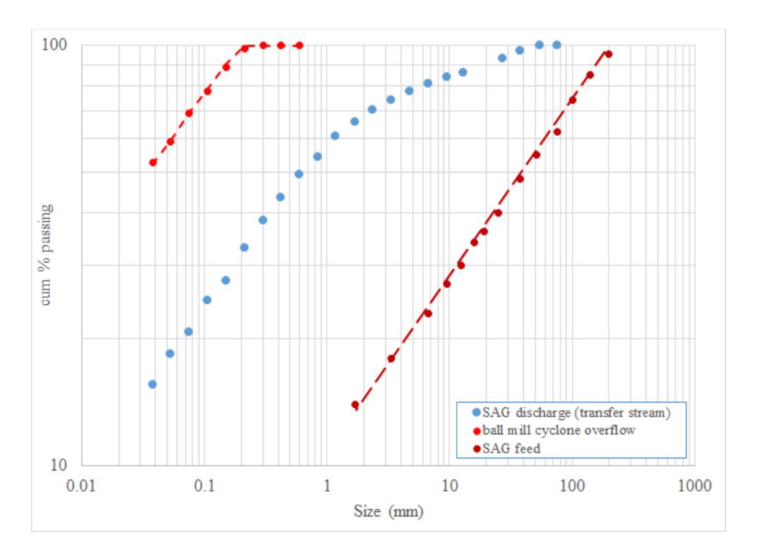
Apart from the fact that there are no equations to predict the transfer size ( \( T_{80} \) ) in Barrett and Allan's approach (eq 10 and 11) and that even though the SPI model has \( T_{80} \) equations, they are highly complex, typically AG/SAG mill circuits' transfer stream size distributions do not follow the strict mathematical requirement of power-based models that they are linear in log-log space and parallel to the feed and final product streams (Morrell, 2011). Figure 1 shows an example which illustrates this. For this reason it is not mathematically appropriate to use the \( T_{80} \) in power-based equations.

One way to overcome this problem is to formulate AG/SAG specific energy models without a \( T_{80} \) term. Typical examples are those developed by Morrell (2006) and OMC (Scinto et al, 2015). Morrell's and OMC's equations (21 and 22 respectively) are compared below. Both are very similar, one depending on the DW_i parameter and the other the (A*b) parameter to represent hardness.

$$ E_{SAG} = K F_{80}^{a} DW_{i}^{b} (1+c(1-e^{-dJ}))^{-1} \phi^{e} f(A_{r}) $$ (21)

$$ E_{SAG} = a K (Axb)^b F_{80}^c (1+d(1-e^{-fJ}))^{-1} \phi^g f(A_r) $$ (22)

where

\( E_{SAG} \) = specific energy at the pinion \( F_{80} \) = 80% passing size of the feed \( DW_i \) = SMC Test drop-weight index

A*b = JK drop-weight test hardness parameters

J = volume of balls (%) \( \phi \) = mill speed (% of critical) \( f(A_r) \) = function of mill aspect ratio

K = function whose value is dependent upon whether a pebble crusher is in-circuit a,b,c,d,e,f,g are constants

Another way to overcome the T ⁸⁰ problem in power-based models is to adjust the distribution in some way so that it conforms to the rules of "linear in log-log space and parallel to the feed and final product streams" then use it in Morrell's general equation (8). This can be done by first decomposing the true transfer size distribution into two distributions which are linear and parallel in log-log space, one which is relatively coarse and one which is relatively fine. This is demonstrated using the data in Figure 1. Figure 2 shows the resulting fitted coarse and fine distributions. In this example combining the 2 distributions using the weighting 55% fine and 45% coarse gives the required overall fit to the true transfer distribution.

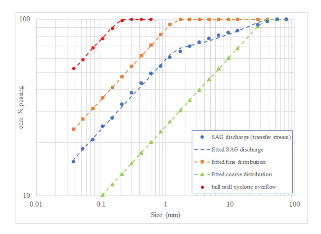
Given that the transfer size distribution can be represented by two distributions which are linear and parallel in log-log space they meet the mathematical requirements for use in power-based equation 8. It therefore follows that there should exist a single distribution, parallel to these two distributions, which, when used in conjunction with equation 8, should give the same answer in terms of specific energy as when the two distributions are combined together. This can be represented mathematically as follows using eq 23:

Let the unknown distribution be called the "Virtual" transfer size distribution and its 80th percent passing size be denoted as "T80VM". The 80th percent passing size of the coarse distribution is denoted as Coarse ⁸⁰ and that of the fine is Fine80. Their respective weighting factors are denoted D ^c and Df. Let it be assumed that it is required to predict the specific energy (ESAG) of a SAG mill with a feed which has an 80th percent passing size denoted as F80. The specific energy equations are as follows:

Using the coarse and fine distributions:

$$ E_{SAG} = 4 M_{ia} (D_c (Coarse_{80}^{f(Coarse_{80})} - F_{80}^{f(F80)}) + D_f (Fine_{80}^{f(Fine_{80})} - F_{80}^{f(F80)})) $$ (23)

Using the "Virtual" distribution:

$$ E_{SAG} = 4 M_{ia} (T_{80VM}^{f(T80v)} - F_{80}^{f(F80)}) $$ (24)

Combining equations 23 and 24 gives:

$$ T_{80VM}^{f(T80v)} = (D_c (Coarse_{80}^{f(Coarse_{80})}) + D_f (Fine_{80}^{f(Fine_{80})})) $$ (25)

As the only unknown in equation 25 is the T80VM its value can be found. To illustrate this the data in Figure 2 are used in the following worked example:

D ^c = 0.45 D ^f = 0.55

Coarse ⁸⁰ = 19084 microns Fine ⁸⁰ = 795 microns

f(Coarse80) = -(0.295+19084/1000000) f(Fine ⁸⁰ ) = -(0.295+795/1000000)

Equation 25 then becomes:

$$ T_{80VM}^{f(780MV)} = 0.45*19084^{-(0.295+19084/1000000)} + 0.55*795^{-(0.295+795/1000000)} $$ (26)

= 0.613

Hence:

$$ T_{80VM}^{-(0.295+T80v/1000000)} = 0.613 $$ (27)

By solution:

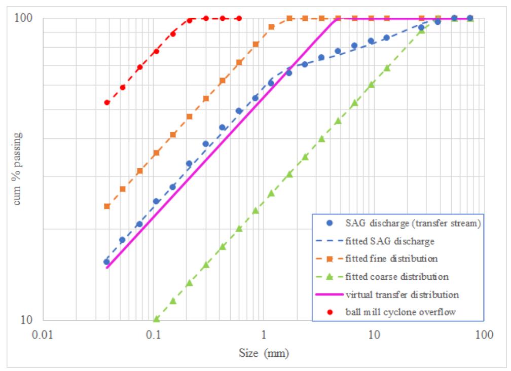
T80VM = 2572 microns

The Virtual transfer size distribution for this example is superimposed on the data from Figure 2 and is presented in Figure 3.

If the T80VM is known then the specific energy of the AG/SAG mill can be predicted from eq. 28, providing the relevant hardness value (Mi) and the feed F ⁸⁰ are known. In such situations the relevant M ⁱ value is the Mia, which is obtained from the SMC Test® .

$$ E_{\text{sag}} = 4*K_1*M_{ia}*(T_{80VM}f^{(T80VM)} - F_{80}f^{(F80)}) $$ (28)

Where K ¹ is 1.0 for all circuits that do not contain a recycle pebble crusher and 0.95 where circuits do have a pebble crusher (Morrell 2008).

In the design situation T80VM needs to be specified for equation 28 to be solved. The transfer size distribution cannot be independently controlled in AG/SAG mill circuits other than those in closed circuit with cyclones or fine screens (Morrell, 2011). As such they cannot be simply specified by the designer with the expectation that in practice the circuit, when built, can be easily "tuned" to match the value. The transfer size that is achieved in practice is a consequence of factors such as aspect ratio, feed size distribution, ball load and whether there is a pebble crusher in the circuit. Hence to determine the transfer size an equation needs to be developed to provide the appropriate associations. Such an equation is given below and was developed empirically from measurements taken from a range of operating circuits:

T80VM	=	d )*Ape*sgf*f(J) K2 *(a*ln(L/D)+b)*exp(c*F80*(L/D) (29)
Where
T80VM	=	80th percent passing size of the virtual transfer size distribution
(L/D)	=	Aspect ratio which is the mill effective grinding length divided by its diameter
F80	=	80th percent passing size of the feed size distribution
Ap	=	aperture of the trommel/screen
sg	=	specific gravity of the ore
f(J)	=	function of ball load volume
K2	=	varies depending on whether the circuit is SAB, SABC-A or SABC-B
a,b,c,d,e,f	=	constants

Model Accuracies

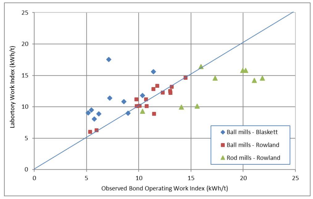
From a designer's viewpoint accuracy has to be evaluated in terms of how near the model's predictions match data from full scale plants. Some published models such as those of Barrett and Allen (eq 10 and 11) provide no information about accuracy. Even Bond himself (eq 2) provided no data concerning accuracy, only quoting in his 1961 Allis Chalmers publication that "Many (equations) are empirical, with numerous constants being derived from experience." However Bond's co-workers at Allis Chalmers such as Rowland (1973) and Flavel and Rimmer (1981) plus a number of other researchers such as Blaskett (1969) and Moore (1982) have published data which reflect the accuracy of Bond's models. Examples can be seen in Figures 4 and 5 which show how well Bond's models predict crusher, rod and ball mill specific energy.

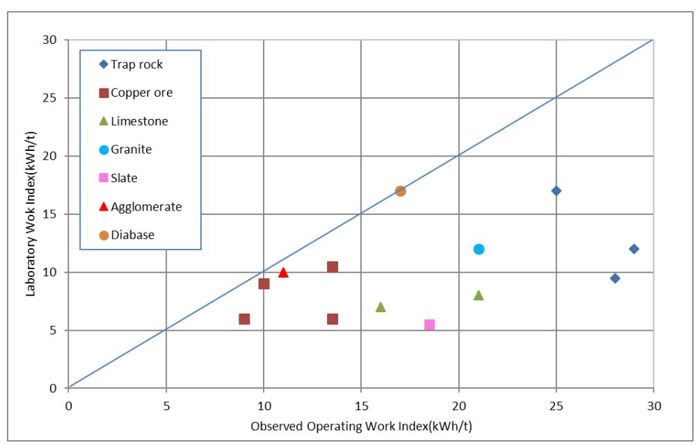
In the case the Bond crushing model the data in Figure 4 show the approach has very poor accuracy and confirms Flavel and Rimmer's conclusions. Flavel and Rimmer claimed that the reason for the poor accuracy was that Bond originally developed his crushing work index test for primary crushers in which the applied specific energy is low (approximately 0.1 kWh/t), but it was not suitable for secondary and tertiary crushers where the applied specific energy was much higher (> 0.25 kWh/t). A contributing cause is the inherent very poor reproducibility of the test as reported by Angove and Dunne (1997) in a study they conducted in which three different samples were sent to several laboratories for Bond crushing work index testing. Results indicated a huge variation in work index values, with maximum values consistently almost double the minimum values. This variation is suspected to be caused by both the lack of standardization in equipment used by different laboratories and the operator sensitivity inherent in the use of the machine. Analysis of the data in Figure 4 indicates that the standard deviation of the differences between observed and predicted values is 22.9% with an overall mean of differences of 39.9%.

With respect to Figure 5, if Rowland's data only are considered, the standard deviation of the differences between observed and predicted specific energies is 9.3% with a mean difference of 1.8%. However, if Blaskett's data are added (and ignoring the one very problematic data set), this standard deviation increases to 25.6% with an overall mean of differences of 16.5%. In the case of the rod mill data, the standard deviation of the differences between observed and predicted specific energies is 12.6% with an overall mean of differences of 21.8%.

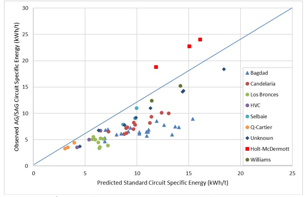
In the case of the SPI models for SAG mills (eq 12-20) Kosick and Bennett (1999) reported the fitting of the empirical factors K and n to data from 13 different. According to Dobby et al. (2001), further data were added to give a total of 26 plants that were used to fit the remaining 23 parameters in the fsag and T ⁸⁰ submodels. According to Amelunxen et al. (2014) the K and n have the values of 5.9 and 0.55 respectively. They used these parameters to compare the observed AG/SAG mill specific energies from 58 data sets from 14 different plants with the predicted values using equation 12 and the fsag term set to unity. The resultant observed and predicted specific energies are given in Figure 6. The obvious considerable scatter in Figure 6 results from the setting of the fsag to unity. Amelunxen et al. (2014) provide guidance as to what values fsag should take and when these values are applied Figure 7 results. Scatter is reduced significantly, though there is a problem with the Holt-McDermott data, a problem that Starkey and Dobby (1996) also noted and stated needed further investigation.

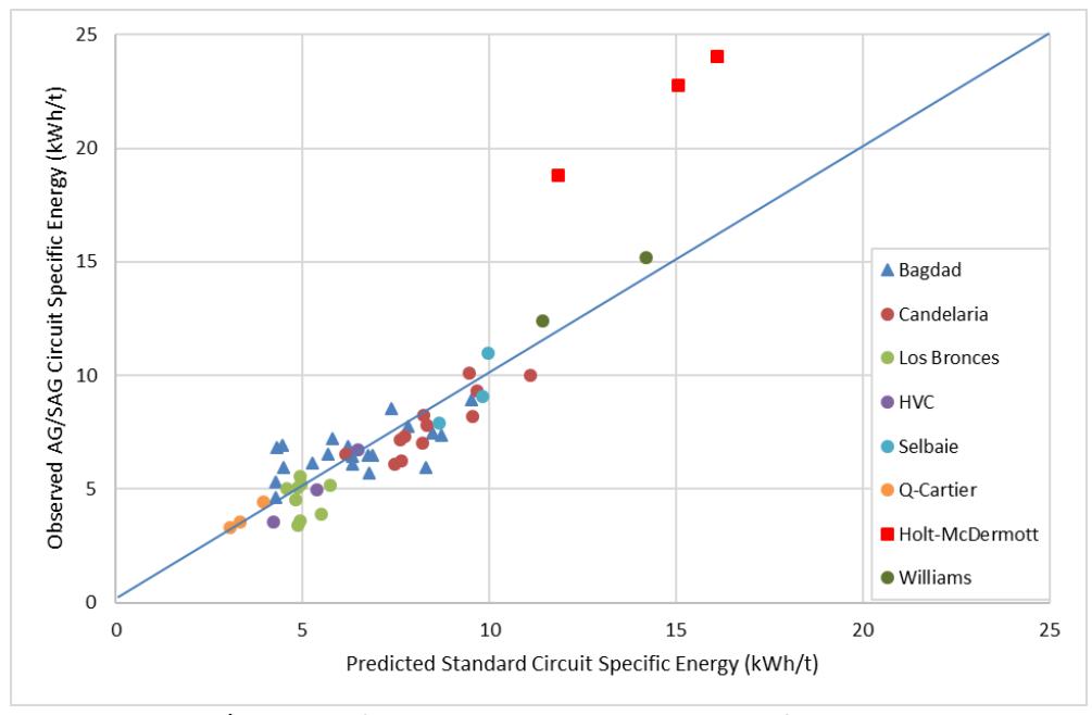
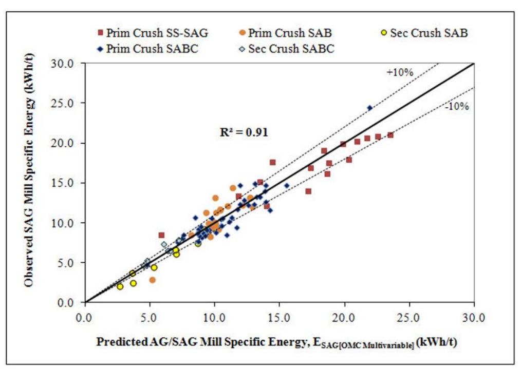
Examination of the statistics associated with the data in Figure 7 indicates that the standard deviation of the differences between the observed and predicted values is 18.9% with a mean of the differences of 0.3%. If the Holt-McDermott data are not included, the results are 17.3% with a mean difference of 2.3%. However, the predicted data in Figure 7 were generated from equations that used the observed T80, not predicted ones, which would be the case in design situations and would increase the scatter in Figure 7 and hence the degree of uncertainty in the predictions. As Amelunxen states, "estimating the transfer size (is) . . . one of the limitations of the (SPI) scale-up methodology ," a limitation that applies to all methodologies requiring knowledge of what the transfer will be. OMC published Figure 8 respectively which show the accuracy of their SAG model (eq22). According to Scinto et al. (2015), the average absolute error of the differences between the observed and predicted AG/SAG mill specific energies is 8.7%. It is estimated that this value is approximately equivalent to a standard deviation of 11.2%, assuming that the mean overall difference between observed and predicted value is approximately zero.

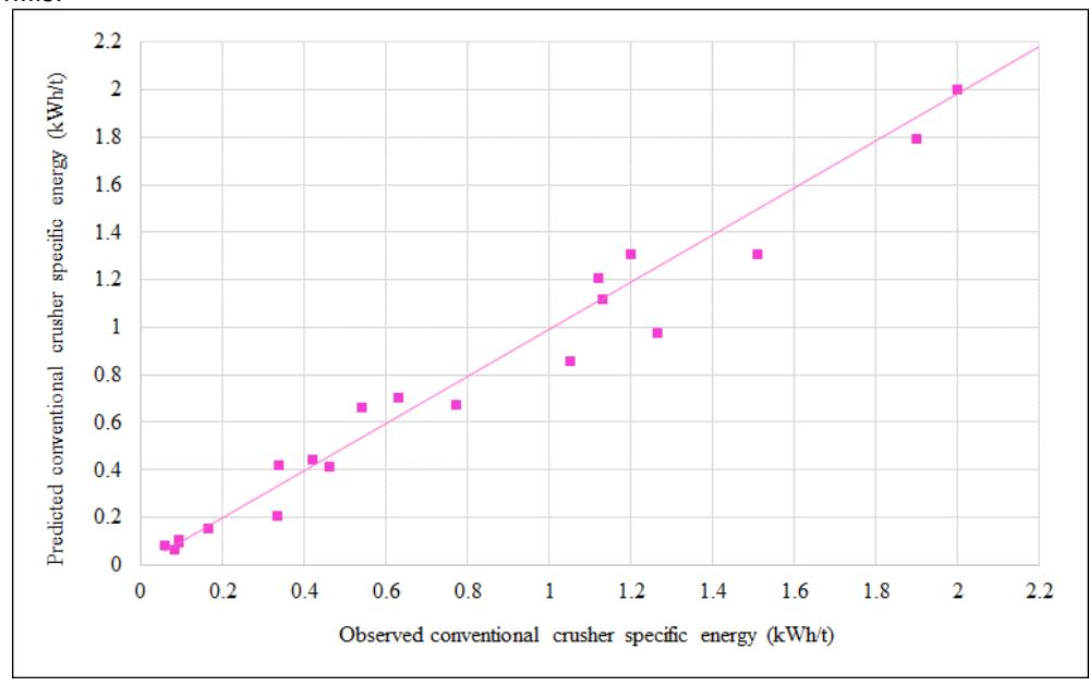
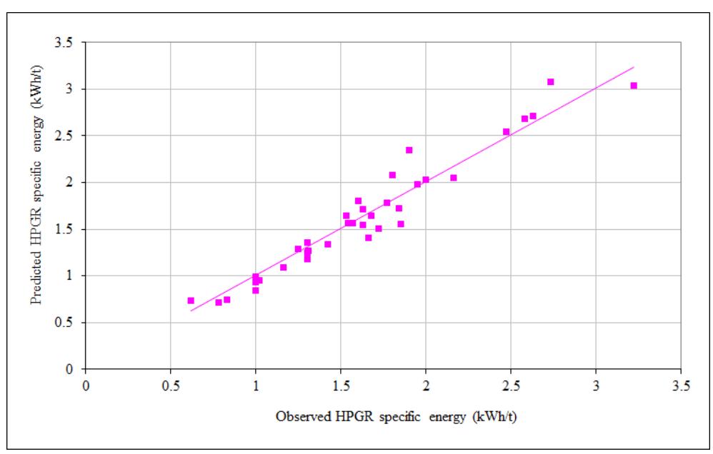
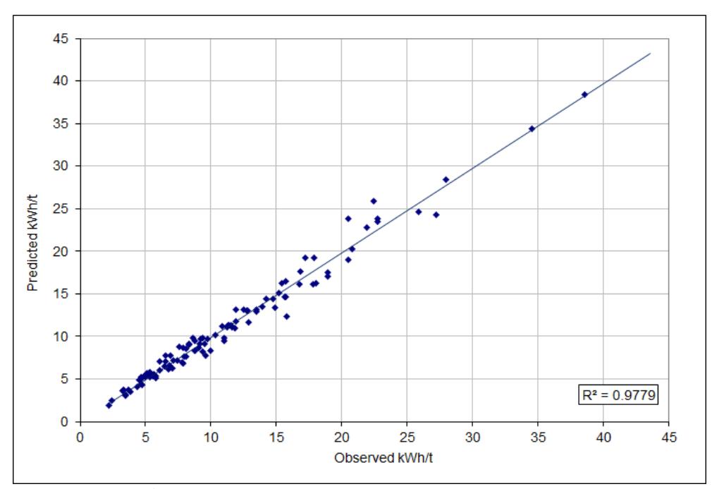
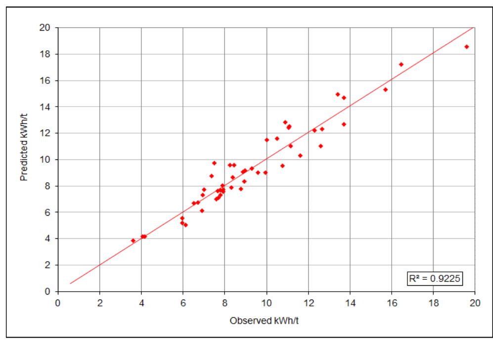
Morrell's equations (8, 21 and 28) have been evaluated against a large data base of operating circuits and their accuracy is demonstrated in Figures 9-12 covering crushing, HPGR, AG/SAG and ball mills respectively. Analysis of the data indicate that the standard deviation of the differences between the observed and predicted values is 18% for crushers, 8.5% for HPGRs, 8.6% for AG/SAG mills and 8.9% for ball mills.

SIMULATION MODELLING

The advent and rapid development of high speed computers provided the opportunity to develop complex models of comminution machines that could execute their calculations very rapidly and which could be linked together such that entire circuits could be simulated. Such models contrast significantly with power-based model and are aimed at reproducing the overall response of comminution machines in terms of throughput, power draw and product size distribution as well as their interaction with other machines in the circuit. By their very nature such models are relatively complex and may have many interactions between the various sub-processes that describe the machine in question, and which without computers would be almost impossible to apply in a reasonable time-frame. Hence in parallel with the development of modern computers, researchers started developing mathematical simulation models of AG/SAG mills, ball mills, crushers and classifiers eg Lynch (1977), Austin et al (1984), Herbst and Fuerstenau (1973), Whiten (1974). Much of the early modelling work was very much academically oriented and there was little benefit to be gained from it by practicing Metallurgists. However as time went on user-friendly interfaces were developed which broadened their appeal and impact. Such developments gave rise to process simulators such as MODSIM, USIMPAC, METSIM, CM-DOCC (Tian et al., 2015) and JKSimMet.

In all cases comminution simulation model researchers relied on what is known as the population balance model (or variants of it) as their mathematical framework as it elegantly encapsulated the size reduction process in many comminution machines. The population balance model was originally introduced by Epstein (1947) and can be represented as follows:

$$ 0 = f_i - p_i + \sum_{j=1}^{i-1} k_j s_j b_{ij} - k_i s_i $$ (30)

where,

f_i = tph of particles of size i in the feed p_i = tph of particles of size i in the product k_i = breakage rate of particles of size i

s ⁱ = mass of particles in the charge of size i

bij = breakage distribution function

Whiten's variant (1974) of the population balance model essentially uses equation 30 but to it he added another equation which enabled the introduction of material transport to be easily incorporated, which greatly aided the development of grate discharge mill models such as those that could be applied to AG/SAG mills. This equation was written:

where

d ⁱ = discharge rate of particles of size i

The simplicity of the above equations is both the source of their greatest strengths but also their greatest weaknesses. Their greatest strengths are their ease of use and great versatility, whilst their greatest weakness is the lack of any physical description of the sub-processes on which they depend. For them to be used successfully, therefore, a series of supplementary models must be developed and linked to them. Even when such sub-processes are developed, invariably there will remain a range of parameters which, for the models to work, must be specified. Considering equations 30 and 31 for example, if a product size distribution and charge is required to be obtained from simulation of a mill grinding a specified feed, then size-distributed parameters ki, bi, and d ⁱ must be specified. In the case of the JKSimMet modelling approach (Napier Munn et al, 1996) the b ⁱ parameters are derived from the A and b values that are obtained from drop-weight or SMC Tests. This leaves the d ⁱ and k ⁱ which, in the early years of development, had to be fitted to data from existing mills. As a consequence of this the use of such models was restricted to process optimisation studies and hence in design situations they were of limited use. However, even though limited to optimisation studies, such models were extremely valuable as they enabled practicing Metallurgists to run and assess strategies to improve plant performance. This cut down significantly the time consuming and potentially costly trial-and-error field experimentation that was the usual methodology up until then. Many models in currently commercially available simulators still suffer from the problem of requiring existing plant data for suitable parameters and hence still have limited use in design projects. The JKSimMet AG/SAG mill "Variable Rates Model" (Morrell and Morrison, 1996) and CM-DOCC's Morrell AG/SAG model (2004) are two exceptions. Both models used a range of operating plant data to determine the dependency of the model parameters on factors such as mill design and operating conditions. An example of the data that was used to develop these dependencies is shown in Figure 13. This illustrates the highly important breakage rate distribution, which changes its shape depending on the design and operating conditions. By mathematically describing how this shape changes, the resultant equations can be used in design situations to predict the required breakage rate parameters for the simulation to be carried out. This gives the Design Metallurgist a very powerful tool as it enables stream mass and size balances to be generated from the chosen circuit and chosen mill sizes and allows him/her to run sensitivity analyses to ensure that target throughputs and grind sizes can achieved under a range of feed and operating conditions. This significantly increases confidence that the chosen circuit and equipment will achieve their specified goals.

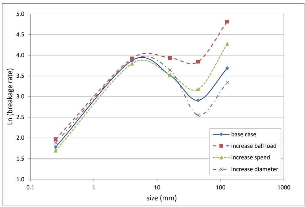
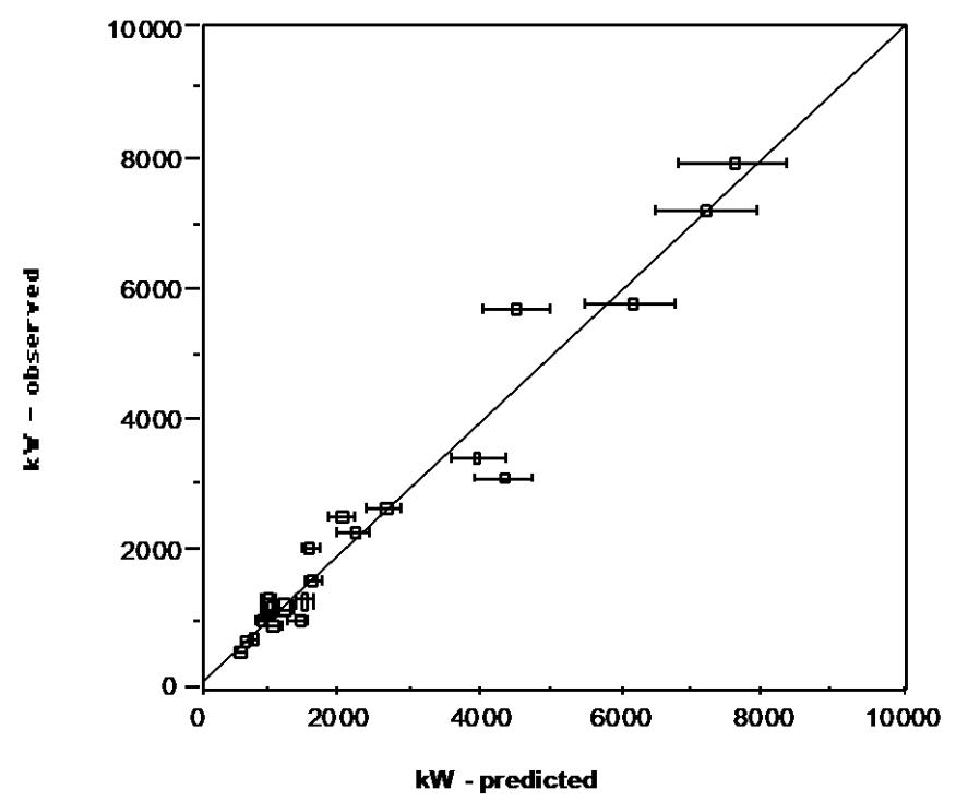
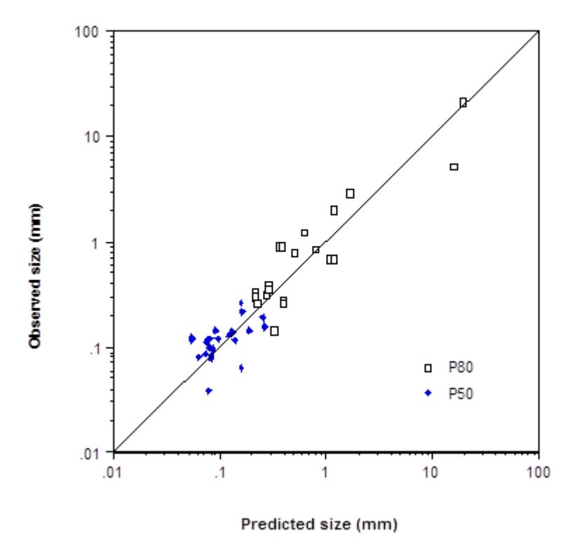
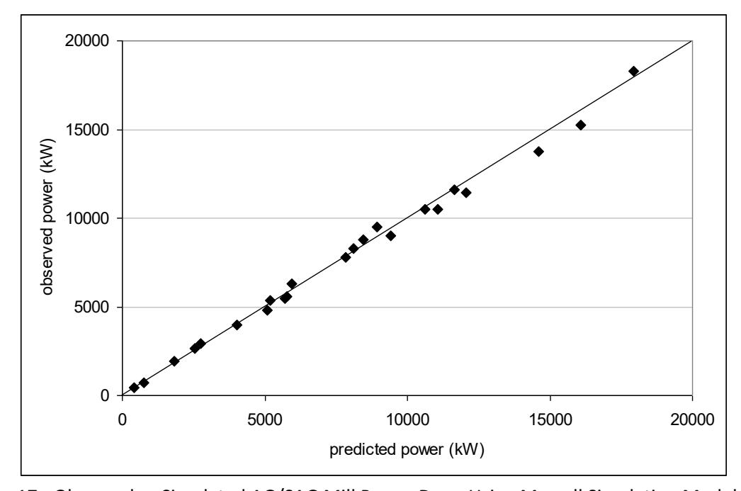
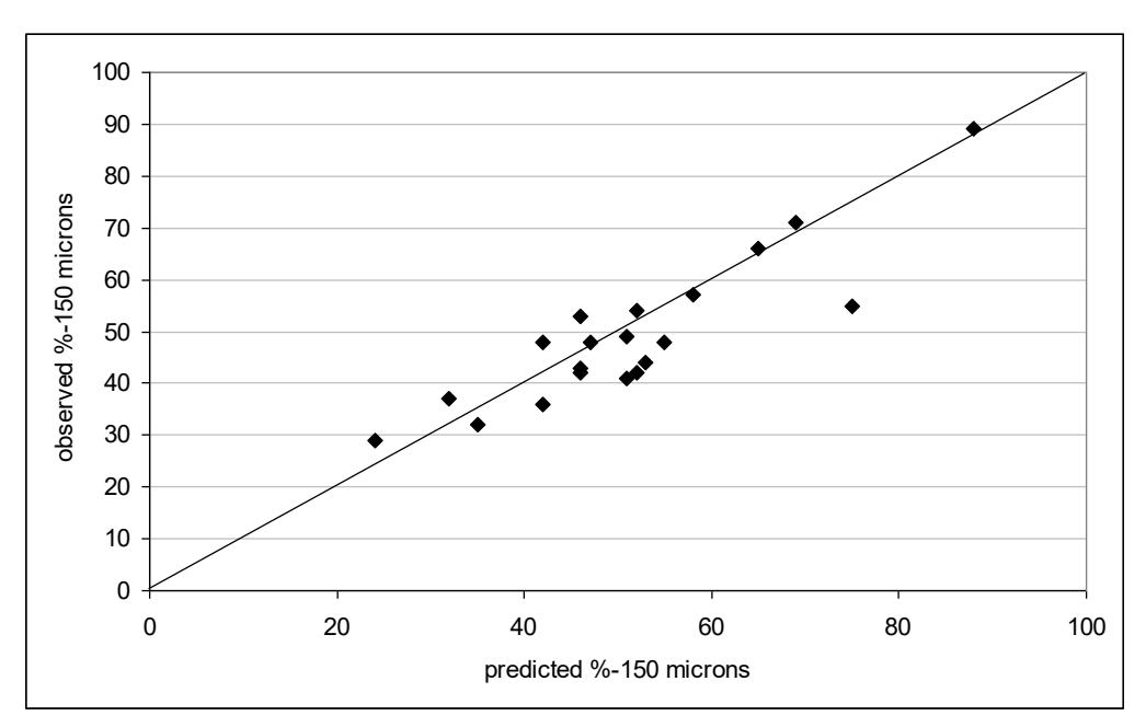
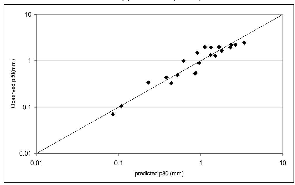
What no model is (regardless of how sophisticated it is), is an expert system that enables Metallurgists with limited knowledge/experience to become " instant experts" by having a simulator at their disposal. At the end of the day models/simulators are just tools and it is incumbent on the user to fully understand how they work, what their limitations are and understand the operational intricacies of the processes that they simulate. In particular knowing the model limitations is important and this can only be established by benchmarking the performance of the models over as wide a range of operating data as possible. According to the published literature this has not often been done, with the exception of the JK Variable Rates and CM-DOCC Morrell models (see Figure 14-19)

The so-called JKMRC "Variable Rates" model is arguably the most commonly used AG/SAG mill simulation model. During its development a total of 18 AG/SAG mills were used for benchmarking purposes (Morrell and Morrison, 1996). This was done by running the model under the same feed conditions as the full scale mill and comparing the power draw of the actual mill with that predicted by the model. The results are shown in Figure 14. The predicted product sizes were also compared with those measured on the plant and are given in Figure 15.

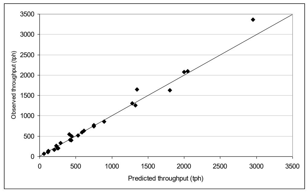
More recently Morrell (2004 ^b ) developed a more advanced AG/SAG model than the Variable Rates one and it was benchmarked using a total of 21 different mills. The model predictions were compared with plant operating data by running the simulation model until it reached the same operating load that was observed on the plant. Comparisons were then made between the simulated throughput and power draw and the observed values. The results are shown in Figures 16 and 17 respectively. Comparisons of the predicted product size and the observed values were also made (Figures 18 and 19).

CONCLUSIONS

Comminution models have come a long way from their beginnings in the mid-1800's when researchers such as von Rittinger first published their ideas relating to so-called power-based models which attempted to relate specific energy to size reduction in comminution machines. Since that time alternative ideas/hypotheses have abounded. However it wasn't until Bond in the mid 1900's that such models were imbedded into a practical methodology that could be of real use to the practicing metallurgist interested in crushing and ball mill circuits. Further advancements followed in the late 1900's and early 2000's with power-based models for AG/SAG mills and HPGR's such as those developed by Morrell. Also in the late 1900's the rapid development of personal computers lead to a similarly rapid development of simulation models such as those in JKSimMet, which provided metallurgists with unprecedented levels of predictive detail when designing circuits. For today's practicing metallurgists there exists a plethora of models to aid in circuit design/equipment selection which may provide him/her with the dilemma of which one(s) to choose. The answer to this is straight forward and lies in the extent to which the model's accuracy has been tested against full-scale data. If it hasn't then there exists a real and significant risk of it producing inaccurate results. If it has been properly evaluated the resultant accuracy statistics will provide the designer with the degree of uncertainty associated with its predictions and this can be catered for within the design to ensure success.

REFERENCES

Austin, L.G., Klimpel, R.R., and Luckie , P.T. 1984. The Process Engineering of Size Reduction: Ball Milling. New York: AIME

Amelunxen, P., Berrios P., and Rodriguez, E. 2014. The SAG grindability index. Miner. Eng. 55:42–51 Barratt D.J. and Allan M.J . 1986. Testing for autogenous and semiautogenous grinding: a designer's point of view, Minerals and Metallurgical Processing, pp.65-74.

Blaskett K.S ., 1969. Estimation of the Power Consumption in Grinding Mills. Proceeding of the Ninth Commonwealth Min. Metall., 3, pp 631-649.

Bond, F.C . (1952) The third theory of comminution. Trans. AIME, vol. 193. pp. 484–494.

Bond, F.C . (1961) Crushing and grinding calculations, Part I-II. Br. Chem. Eng., vol. 6.

Bond, F.C., 1961 (revised 1962). Crushing and Grinding Calculations. Allis-Chalmers publication O7R9235B

Charles, R. J . (1957). Energy-size reduction relationships in comminution. Transactions of the AIME, 9(1), 80-8.

Dobby, G., Bennett, C., and Kosick , G. 2001. Advances in SAG circuit design and simulation applied to the Mine Block Model. In Proceedings of the Conference on International Autogenous and Semi-Autogenous Grinding Technology 2001. Vol. 4. Vancouver, BC: Mining and Mineral Process Engineering, University of British Columbia.

Epstein B. (1947) The Material Description of Certain Breakage Mechanisms Leading to the Logarithmic-normal Distribution. J Franklin Inst, pp244-471

Flavel M. D. and Rimmer H.W ., 1981. Particle Breakage Studies in an Impact Environment. Proc. SME-AIME Annual Meeting, Chicago.

Global Mining Guidelines Group (2016a).

https://gmggroup.org/wpcontent/uploads/2018/06/Guidelines_Bond-Efficiency-REV-2018.pdf Global Mining Guidelines Group (2016b).

https://gmggroup.org/wp-content/uploads/2018/06/Guidelines_-Morrell-REV-2018.pdf

Herbst, L.A., and Fuerstenau, D.W. 1973. Mathematical simulation of dry ball milling using specific power information. Trans. AIME 254:343–348

Holmes, J.A . (1957). A Contribution to the Study of Comminution – A Modified Form of Kick's Law. Trans. Instn Chem. Engrs, Vol. 35, pp 126-157

Hukki, R.T . (1962) Proposal for a Solomonic Settlement Between the Theories of von Rittinger, Kick, and Bond. Trans. AIME, 223, pp. 403–408.

Kick, F . (1885) Das Gesetz der proportionalen Widerstande und seine anwendung felix. Leipzig, Germany.

Kosick, G.A., and Bennett, C . 1999. The value of ore body power requirement profiles for SAG circuit design. In Proceedings of the 31 st Annual Meeting of the Canadian Mineral Processors , Ottawa, ON: Canadian Mineral Processors.

Lynch, A.J . (1977). Mineral Crushing and Grinding Circuits: Their Simulation, Optimisation, Design and Control. Amsterdam, Netherlands: Elsevier Scientific

Moore D. C., 1982. Prediction of Crusher Power Requirements and Product Size Analysis. Design and Installation of Comminution Circuits, AIME, Chapter 14, pp218-227

Morrell, S. and Morrison, R . (1996). AG and SAG mill circuit selection and design by simulation. Proc SAG '96, Vancouver, pp 769-790

Morrell, S. (2004a) An alternative energy-size relationship to that proposed by Bond for the design and optimisation of grinding circuits, International Journal of Minerals Processing, vol. 74. pp. 133–141.

Morrell, S .,2004b, A new autogenous and semi-autogenous mill model for scale-up, design, and optimisation. Minerals Engineering 17 (2004) 437-445

Morrell, S., 2009, Predicting the overall specific energy requirement of crushing, high pressure grinding roll and tumbling mill circuits, Minerals Engineering,

Volume 22, Issue 6, May, Pages 544-549

Morrell, S., 2010, Predicting the specific energy required for size reduction of relatively coarse feeds in conventional crushers and high pressure grinding rolls, minerals engineering Volume 23, Issue 2, January, Pages 151-153

Morrell, S ., 2011. The Appropriateness of the Transfer Size in AG and SAG Mill Circuit Design, Proc International Autogenous and Semi Autogenous Grinding Technology,Vancouver,paper #153

Neumaier A ,(2004) Mathematical Model Building, Chapter 3 in: Modeling Languages in Mathematical Optimization (J. Kallrath, ed.), Applied Optimization, Vol. 88, Kluwer, Boston

von Rittinger , R.P. (1967) Lehrbuch der Aufbereitungskunde. Ernst and Korn, Berlin, Germany.

Rowland C.A. Jnr . 1973., in. Comparison of work indices calculated from operating data with those from laboratory test data in. . Proc. 10th IMPC, pp 47-61

Rowland Jr C. A . 1982. Selection of rod mills, ball mills, pebble mills and regrind mills. Design and installation of comminution circuits (Eds Mular and Jergensen), SME/AIME, New York, 393-438.

Scinto P., Festa A and Putland B ., 2015. OMC Power-based Comminution Calculations for Design, Modelling and Circuit Optimisation, Proc. 47th CMP Conference, Ottawa

Starkey, J., and Dobby, G. 1996. Application of the Minnovex SAG Power Index at five Canadian SAG plants. In Proceedings of the Conference on International Autogenous and Semi-Autogenous Grinding Technology 1996. Vancouver, BC: Mining and Mineral Process Engineering, University of British Columbia. pp. 110–123.

Tian, J., S, Morrell S., and Wang E . 2015. Design and Optimization of Comminution Circuits Using CITIC SMCC's Integrated Software – " CM-DOCC ". Proc Procemin, Santiago, Chile

Verschaffel,L., Greer,B. and De Corte E . (2002) Everyday Knowledge and Mathematical Modeling of School Word Problems. In book: Symbolizing, Modeling and Tool Use in Mathematics Education. DOI: 10.1007/978-94-017-3194-2_16

Walker, W.H., Lewis, W.K., McAdams , W.H., and Gilliland, E.R. (1937) Principles of Chemical Engineering. McGraw-Hill, NY, USA.

Whiten, W.J . 1974. A matrix theory of comminution machines. Chem. Eng. Sci. 29:588–599.