



The content on this page was automatically generated from the PDF publication document and may contain errors or inaccuracies. Please refer to the original PDF for the most accurate information.
MODELLING THE INFLUENCE ON POWER DRAW OF THE SLURRY PHASE IN AUTOGENOUS (AG), SEMI-AUTOGENOUS (SAG) AND BALL MILLS
S.Morrell
Citic SMCC Process Technology Pty Ltd PO Box 337, Indooroopilly Centre Queensland 4068 Australia
The slurry level in AG/SAG and ball mills has an influence on their power draw, which in some instances can be profound. This is particularly the case with so-called slurry pooling in AG/SAG mills which can result in significant lowering of power draw. From a predictive viewpoint there are currently no published models that explicitly describe the influence of slurry level on power draw and the relationship between slurry level, slurry flow and pulp lifter design. Citic SMCC Process Technology Pty Ltd has developed such a model and in this paper its structure is described. Examples are given of both AG/SAG and ball mills of how the model responds to changes in slurry level. These examples are used to explain the observed phenomena of slurry pooling and the decrease in power draw observed in ball mills after startup when feed is first introduced into the mill.
Keywords: SAG Milling, Comminution
1. Introduction
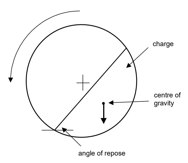
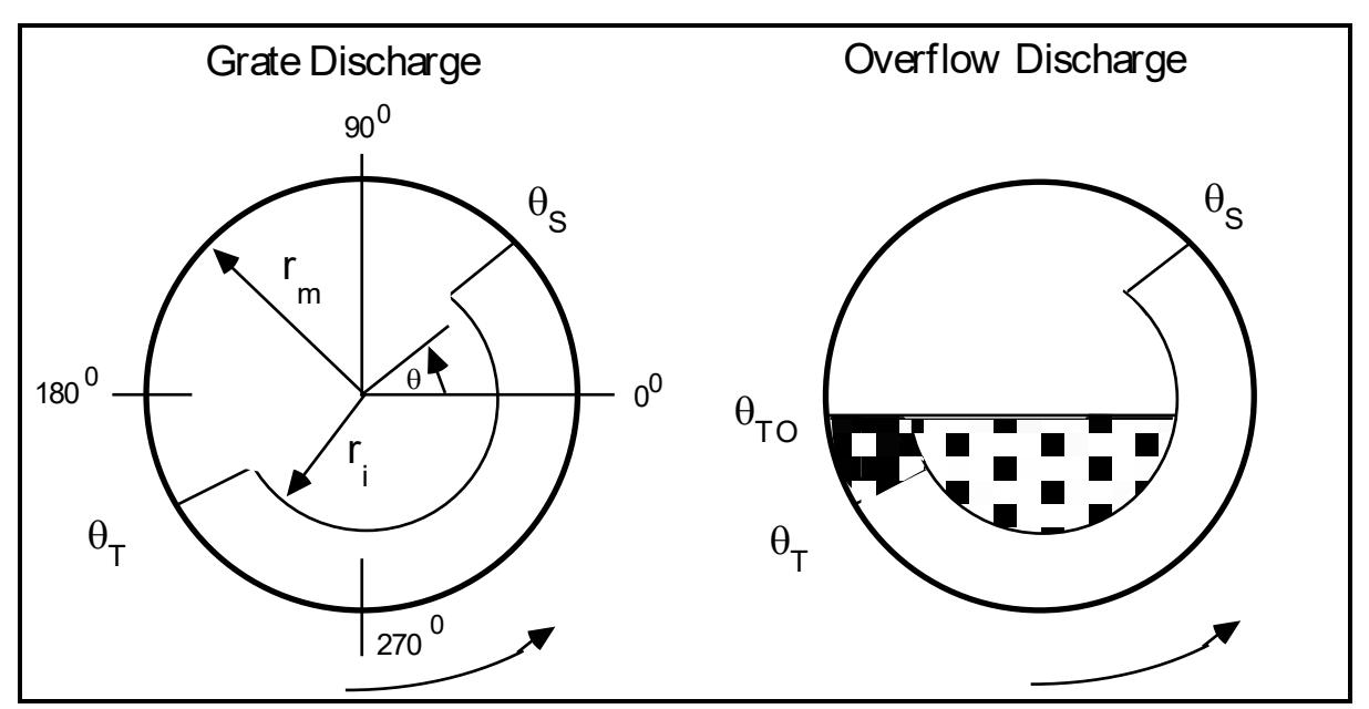
If one looks back over the last 70 years or so there is a fairly common theme to most of tumbling mill power draw models (Bond, 1962, Hogg and Fuerstenau, 1972, Arbiter and Harris, 1982, Austin, 1990). This is that the models used the charge shape shown in Figure 1 in which it was assumed that all particles moved with same rotational rate and that the slurry phase was not explicitly considered. There also appears to have been the view that different models were required for ball mills and AG/SAG mills. This view was perhaps driven by the fact that the early models were developed at a time when AG/SAG mills were almost nonexistent and hence these models simply considered the ball charge only, which, if these models were to be applied to ball mills only is not an unreasonable assumption. Morrell (1996a) found that in fact only one model is required to describe all tumbling mills, whether they are rod mills, ball mills or AG/SAG mills. In its original form Morrell's model used a different media charge shape to that in Figure 1 (Morrell, 1992) and was configured to consider the cases where slurry was contained within the grinding charge as in a typical grate discharge AG/SAG mill (Figure 2a) or where it additionally formed a large slurry pool as occurs in all overflow ball mills (Figure 2b)(Morrell, 1993, 1996a). However, from experience gained with single stage AG/SAG mills it became clear that even grate discharge mills can accumulate slurry at the toe of the charge and this can considerably affect power draw depending on the extent of the slurry pool (Morrell, 1989, Morrell and Kojovic, 1996). Hence it can be concluded that the extent of the slurry phase can have a significant impact on power draw and therefore should be explicitly described if a model is to be as accurate as possible. This paper describes how Citic SMCC Process Technology's (Citic SMCC) power model, which has been developed from Morrell's earlier published work, incorporates the slurry phase.
2. Model Structure
2.1 General
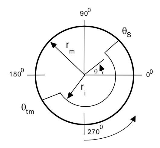
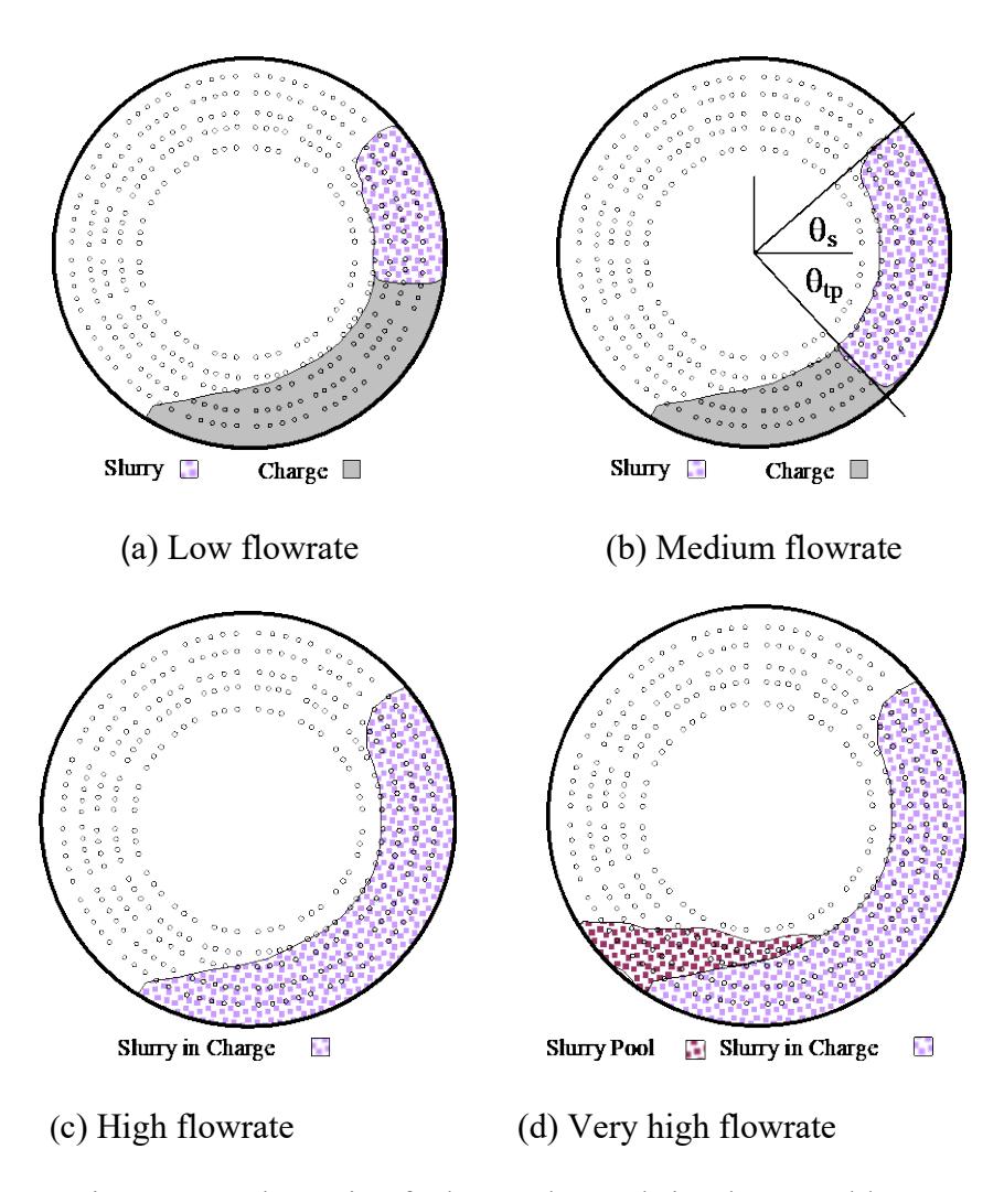
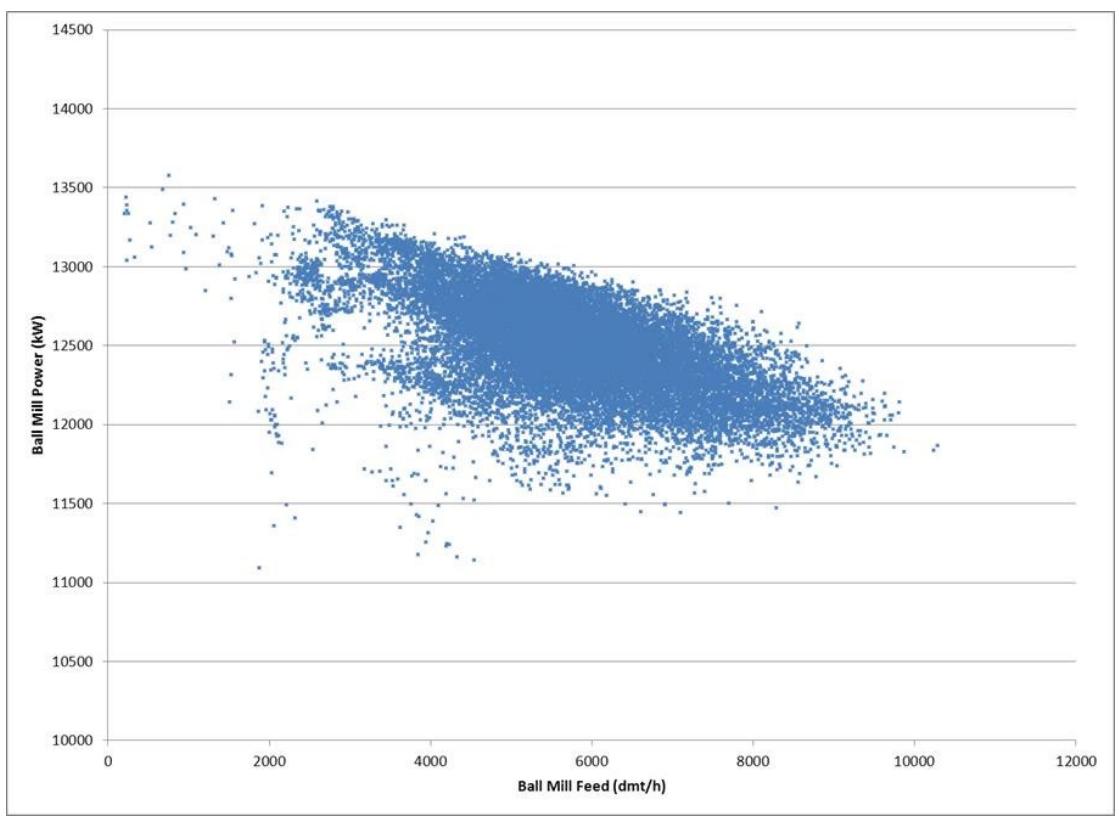
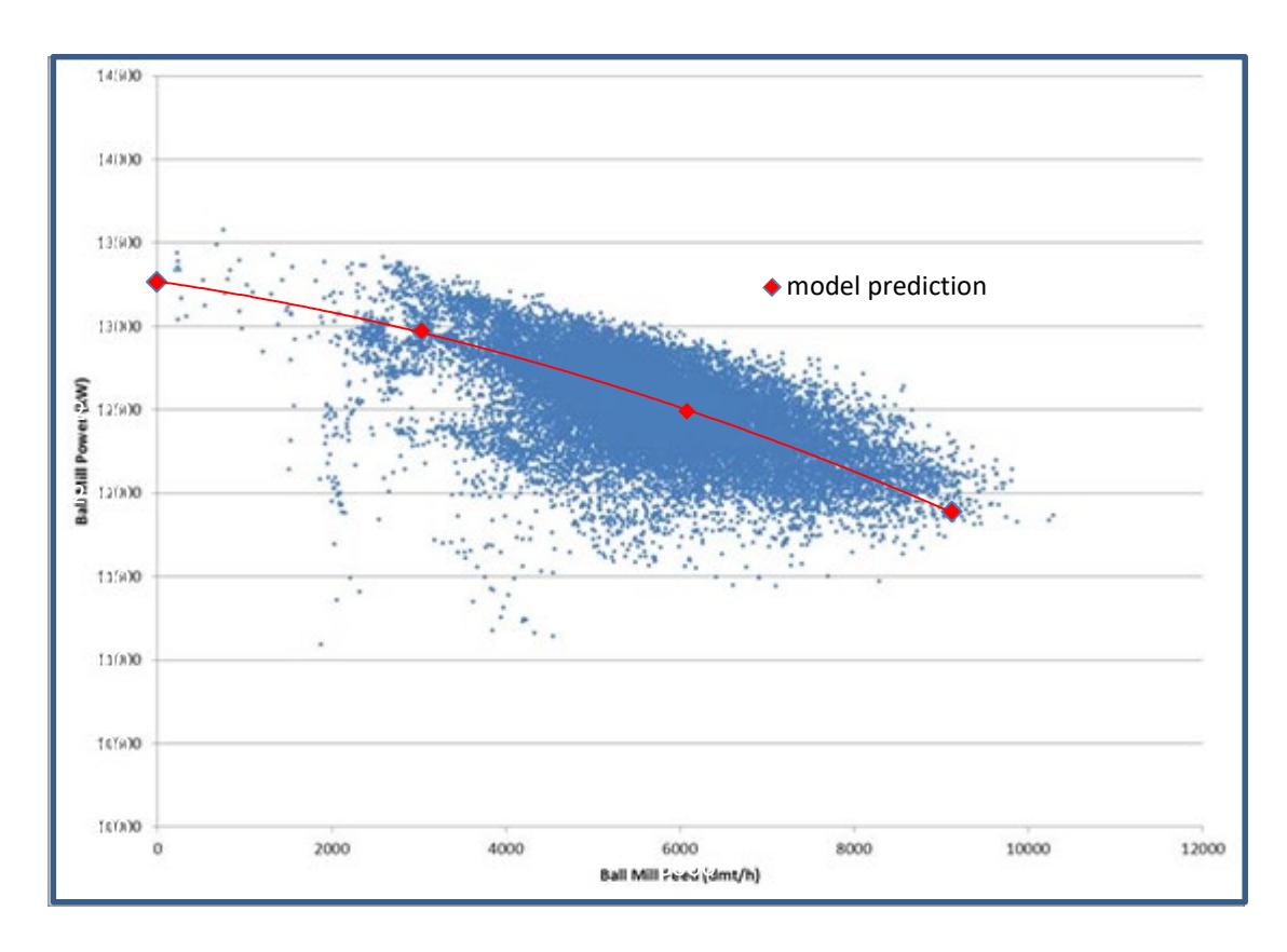
As per Morrell's original model structure, the grinding media part of the charge (rocks and/or ball) is configured as per Figure 3. When a mill is in operation the slurry portion of the charge occupies the grinding media interstices. However, it is not uniformly dispersed but fills the interstices from the shoulder down towards the toe of the grinding media charge (Latchireddi and Morrell, 2003). This it does in response to changes in the slurry flowrate. The toe of the slurry portion of the charge is therefore not necessarily coincident with that of the grinding media. This is illustrated schematically in Figure 4, which shows the movement of the slurry toe as flowrate increases. If the flowrate is high enough a slurry pool forms (Figure 4d) in which case the slurry toe effectively extends beyond the grinding media toe. This causes the power draw to fall as the slurry toe effectively aids in the rotation of the mill. In overflow ball mills this slurry toe extend up to at least the point where it can overflow out of the discharge trunnion. As flow requires a gradient, the slurry toe position in an overflow ball mill will actually be higher than the lowest point of the discharge trunnion and as flow increases the slurry toe will become progressively higher. This situation occurs in all overflow discharge ball mills and gives rise to the lower power draw which is usually seen in overflow ball mills compared to similar-sized grate discharge units and also gives rise to the progressive decrease in power as feedrate increases. This decrease in power draw is typically not great, other than in extreme cases. An example of this phenomenon is seen in Figure 5. The figure shows online data from an operating plant collected over a relatively long period. Scatter in the data is clear and is typical of all real operating data. However, the trend is clear in that as ball mill feedrate increases the power draw falls. As can be seen the average power draw is about 12.5 MW and occurs at a feedrate (new feed plus recycle) of about 6000 t/hr. Over a wide range of feedrates about the mean value of 6000 tph the power draw varies by only +/- 5%. Of note also in Figure 5 is the power draw at zero feedrate, which has the highest value of all. This phenomenon is also common and is explainable by the fact that the slurry pool is at its lowest point and at its lowest density). Its influence depressing power draw is therefore at its lowest.
2.2. Equations
The approach adopted in the Citic SMCC model to handle the slurry phase is to predict its power draw separately to the grinding media phase (balls/rocks), then add the powers of each phase together to obtain the total power draw. Using an energy balance approach, where power is taken to be the rate at which potential and kinetic energy is imparted to the charge, equation 1 was therefore developed for the cylindrical section of the mill. From this equation it can be seen that the power associated with the rock/ball charge is calculated separately from the slurry, the total power being the sum of both. Some mills have conical end-sections and, as they also draw power, have to be included if accurate predictions are to be obtained. This is easily done by using the same approach that Morrell adopted in his original model (1996a).
$$ P_{cylinder} = KL \int_{r_i}^{r_m} (V_r(\rho_m(rg(\sin\theta_s - \sin\theta_{tm}) + 0.5V_r^2) + \rho_p(rg(\sin\theta_s - \sin\theta_{tp}) + 0.5V_r^2)))dr $$ (1)
Where,
\( P_{\text{cylinder}} = \text{power drawn by the charge (net)} \)
K = lumped parameter (constant)
L = length of cylindrical section of the mill inside liners
P = power delivered to the charge (net power)
r = radial position
\( r_i \) = radial position of charge inner surface
rm = radius of mill inside liners
\( V_r \) = tangential velocity of a particle at radial distance r
\( \theta_{\rm S} \) = angular displacement of shoulder position at the mill shell
θtm = angular displacement of the grinding media (rocks and balls) toe position at the mill shell
θtp = angular displacement of the pulp (slurry) toe position at the mill shell (see Figure 4b); for overflow ball mills θtp = θto (see Figure 2b)
ρm = density of rock/ball charge (excluding pulp)
ρp = density of pulp phase
The density of the pulp phase (ρp) is assumed to be the same as the discharge density of the slurry. The density of the rock/ball charge (ρm) is estimated using the following equation:
Where,
Jt = total fractional static volumetric filling (including voids) of balls and rocks
Jb = fractional static volumetric filling (including voids) of balls
ρo = density of rock in the mill
ρb = density of steel media in the mill (usually taken as 7.8 tonnes/cu.m)
ε = dynamic void fraction in the ball/rock media
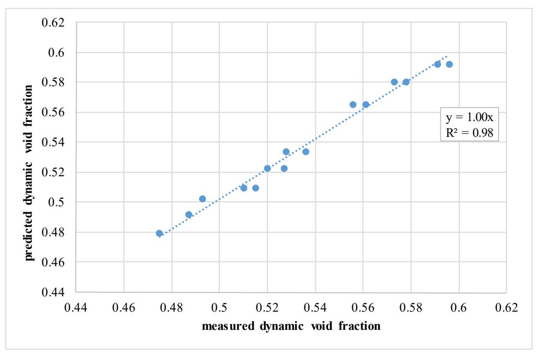
The parameter ε represents the fractional voidage in the charge in the mill whilst it is motion and differs from the static fractional voidage which is normally assumed to be constant at 0.4. Experiments by Latchireddi (2002) showed that the fractional voidage of the charge when it is being tumbled In a mill is not constant and can vary over the range 0.45-0.6, the magnitude being dictated by the speed of rotation of the mill and the grinding media load volume. Higher speeds were found to increase the voidage whilst the grinding media load had the opposite effect. The following equation was fitted to his data to predict ε:
$$ \varepsilon = 0.45*Jt^{-0.15}*\phi^{0.087} $$ (3)
Where,
φ = fraction of critical speed
Jt = total fractional static volumetric filling (including voids) of balls and rocks
The fit of equation 3 to Latchireddi's data is shown in Figure 6.
Equation 1 describes the power draw by the charge (net power) and does not explicitly include electrical losses across the motor as well as the power required to overcome friction in the bearings and losses in gearboxes/reducers as well as in the gear/pinion coupling, where the mill has a gear-and-pinion drive. Note that this definition of net power is not the same as the "power at pinion". The power at pinion cannot normally be measured other than in some pilot mills and is a value which is estimated from assumptions about the energy losses of various components in the drive train. Theoretically it is the power delivered to the pinion shaft in gear-and-pinion drives. As such it is meant to account for electrical motor and gearbox/reducer energy losses only but does not include the energy losses associated with the pinion gear/ring gear coupling nor bearings.
In practice the only power draw that is usually measured in full scale plants is the metered or gross power, ie motor input power. The difference between motor input and net power draw in a mill is due to losses associated with various electrical and mechanical components. The main losses occur in the motor, gearing and bearings. None of these remains constant over the mill's full operating range. Some, however, may have a fixed component - for example, losses in the bearings due to friction will be dictated by the weight of the mill when empty (a fixed component, though even this will vary as liners and lifters wear) and the weight of the mill charge (a variable component). In most, if not all, full-scale operating plants the only data that will be measured is gross power and/or current. In rare cases no-load power (the gross power drawn by the mill when running empty) will be known from commissioning or maintenance records. Alternatively, if the mill has been emptied for relining, the no-load power is sometimes recorded at start-up. Such data indicate the magnitude of some of the power-loss components. Given the need to properly validate the model through comparison of measured and predicted values, the power model must also predict motor input power. Therefore to do so the Citic SMCC model is configured as follows:
$$ Motor input power = No-load power + Net power $$ (4)
Where net power is given by equation 1. A further equation is therefore required which predicts no-load power. The semi-empirical no-load power equation form proposed by Morrell (1996a, Napier-Munn et al, (1996)) is used for this purpose (Equation 5), though it has been modified slightly on the basis of additional data and was developed with the aid of no-load power measurements from a range of plants including pilot mills and mills up to 40ft in diameter.
No-load Power (kW) = $$ \kappa (D^{2.5} \phi (0.667L_d + L))^{0.82} $$ (5)
where κ = 2.13 for gear and pinion drives and 1.28 for gearless drives
D = mill diameter
L = length of cylindrical section
Ld = length of cone end
φ = fraction of critical speed
Clearly to solve the integral in equation 1 it is necessary to have relationships which predict values for parameters such as θs,θtm, θtp,Vr, and ri. With the exception of θtp all of these relationships are provided by Morrell (1993, 1996a) and Napier-Munn et al (1996). The equations relating these parameters to operating conditions and how they vary with radial position (r) were obtained by measurements made from images captured from a rotating glassended mill which was operated at a range of speeds and with a range of grinding media loads. This leaves the lumped parameter (K), which needs to be estimated by fitting it to data from operating mills. Such data were sourced from Citic SMCC's data base and represent 146 ball, AG and SAG mills. In all cases the data sets are operating mills where the ball and rock levels were measured as well as the associated operational power draws (motor input powers). The lumped parameter (K) accounts for energy losses due to sound, heat generated within the charge due to sliding friction, rock breakage due to attrition/abrasion, rotation of the grinding media plus some of the variable losses in the mechanical/electrical drive train not accounted for by the No-load equation.
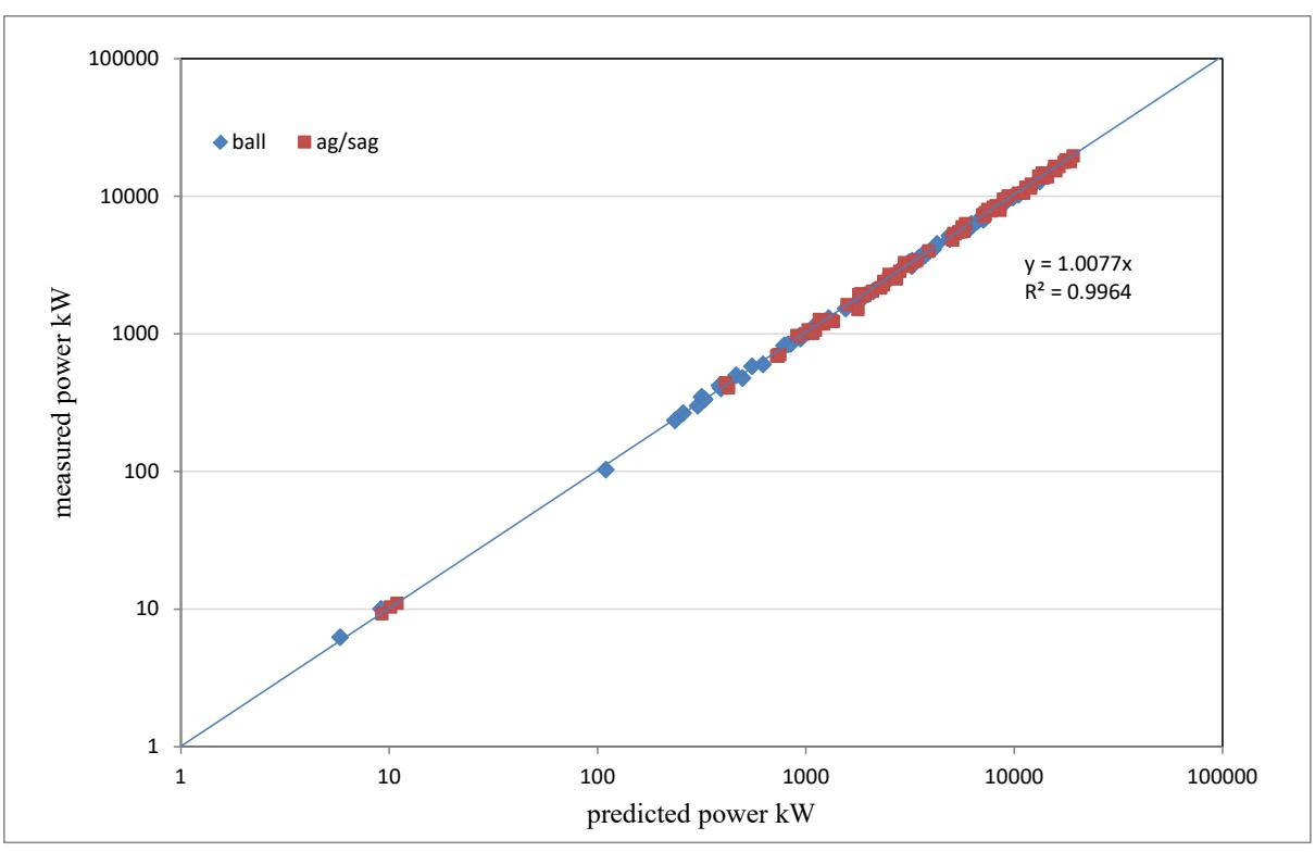
In the vast majority of situations mills are operated in a "normal" regime, eg the AG/SAG mill does not have a slurry pool or the ball mill slurry flowrate is the result of a recycle load which is not excessive. In such cases good predictive results can be obtained by setting θtp to the same value as θtm for AG/SAG mills (this is equivalent to assuming all the interstices are just filled with slurry), and for overflow ball mills a fixed value of θto can be used as proposed by Morrell (1993). When this approach is adopted and only mills which are operating in a "normal" regime are considered, the results given in Figure 7 are obtained. Mills range in size from pilot units to the largest mills currently in operation. The precision of the model as measured by the standard deviation of the relative error is 4%.
3. Predicting the Position of the Slurry Phase ( θ tp)
3.1 Influence of the Slurry Phase
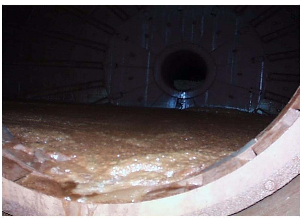
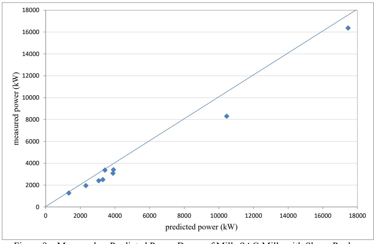
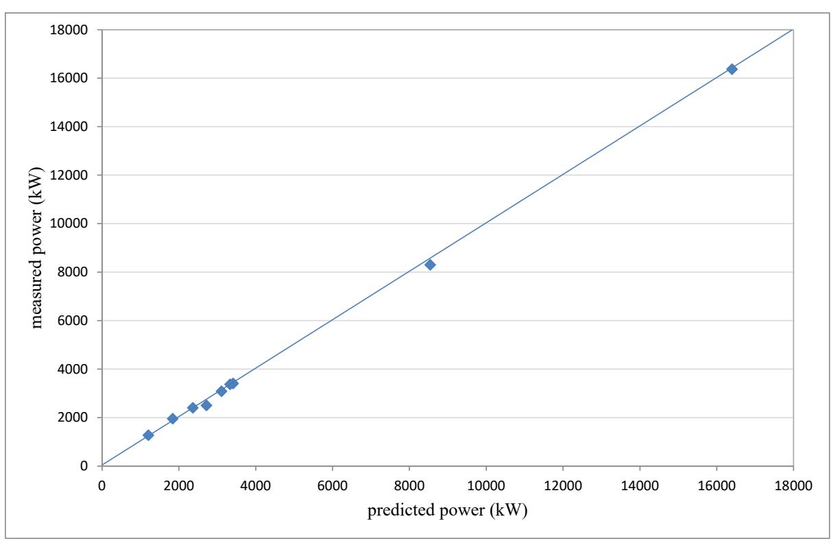
As mentioned in the previous section, providing the mill is operating in a reasonably normal manner, simple approximations of the extent and position of the slurry phase lead to good predictions of the power draw. However, there are situations where, for various reasons, mills operate under unusual conditions and as a result their power response is atypical. Figure 8 is a picture of such a (SAG) mill in which a large slurry pool was forming during operation. Citic SMCC has 9 SAG mill data sets from mills which were found to be operating with varying degrees of slurry pooling. If it is assumed that the mills were operating normally, ie without slurry pooling and θtp = θtm, then the predicted power draws as compared to the measured values are as shown also in Figure 9. As can be seen the measured powers are lower than the predicted values, some values being considerably different (up to 25% lower). However, if the measured slurry pool volumes are used to estimate the true value of θtp and the power model is re-run, then the results shown in Figure 10 are obtained. As can be seen good agreement between the model and the measured power draw is obtained.
3.2 Predicting \( \theta_{tp} \) in Grate Discharge Mills
The challenge in modelling power draw, apart from accurately describing the slurry phase influence on power draw where the slurry volume is known, is to predict the slurry phase volume in the first instance from information on the design of the mill and the slurry flowrate out of the mill. A relationship between slurry flow and slurry volume (so-called hold up) is therefore required. Citic SMCC's slurry flow model for AG/SAG mills (grate discharge mills) was constructed using the approach originally adopted by Morrell and Stephenson (1996) who related the volume of slurry held-up in the mill to its rate of flow out of the grates. Morrell and Stephenson incorporated the effects of grate design, mill speed and charge volume. However, the range of grate designs they used for their experimental programme was very limited and, more importantly, did not take into account the effect of pulp lifters. Latchireddi and Morrell (2003a, 2003b) conducted a detailed laboratory and pilot study of the influence of grate design and pulp lifters on the slurry flow – hold-up relationship and their results were then used to revise Morrell's original equation and incorporate the influence of pulp lifter depth ( \( \lambda \) ). The result was the following general equation:
$$ J_{s} = \eta \gamma^{n_{1}} A^{n_{2}} J_{t}^{n_{3}} \phi^{n_{4}} Q^{n_{5}} D^{n_{5}} $$ $$ \tag{6} $$
Where,
\( J_s \) = the net fractional slurry hold-up inside the mill
A = fractional open area
\( J_t \) = fractional grinding media volume
φ = fraction of critical speed Q = slurry discharge flowrate
\( \gamma \) = mean relative radial position of the grate holes
\( \eta \) = coefficient of resistance which is expected to be a function of viscosity
\( n_1 \) - \( n_6 \) = model parameters
The value of \( \gamma \) is a weighted radial position, which is expressed as a fraction of the mill radius and is calculated using the formula:
Where,
\( a_i \) = open area of all holes at a radial position \( r_i \)
\( r_m \) = radius of mill inside the liners
The parameter values \( n_1 \) - \( n_6 \) and \( \eta \) were found to be functions of pulp lifter size and were all modelled using the following general equation (Morrell and Latchireddi; 2000):
Where,
ng = parameter values for grate-only condition
\( k_i, k_i = constants \)
\( \lambda \) = depth of the pulp lifter expressed as a fraction of mill diameter
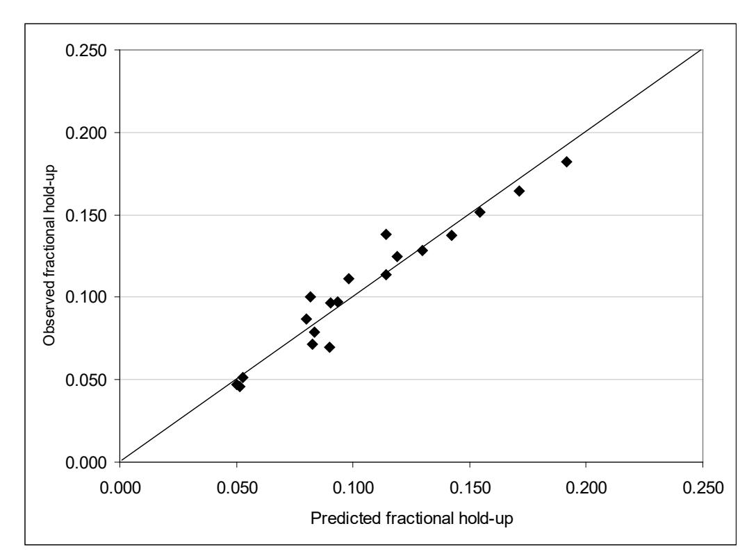
The parameters in the above equations were fitted to over 760 laboratory and pilot mill data sets and 19 full scale mill data sets. The fit of the equations to the full-scale mill data sets are shown in Figure 11.
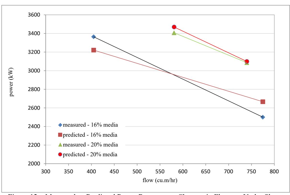
Once the slurry hold-up has been estimated using equations 6-8 the model then determines how much of the interstices (voidage) in the grinding media part of the charge will be occupied by this slurry when the mill is in operation. Using the concept that the voidage in the grinding media is progressively filled from the shoulder down to the toe, the slurry toe position, θtp , can then be determined and used to predict the power draw using equation 1. The extent to which the combination of the slurry hold-up and power draw models are able to reproduce measured behaviour is illustrated in Figure 12 using data from an single stage AG mill in which the flow rates varied yet the media charge volume remained approximately the same. The mill was operating with a slurry pool and therefore as flowrate increased the pool volume increased and hence power draw decreased. As can be seen the predicted power draw behaviour matches the measured response quite well.
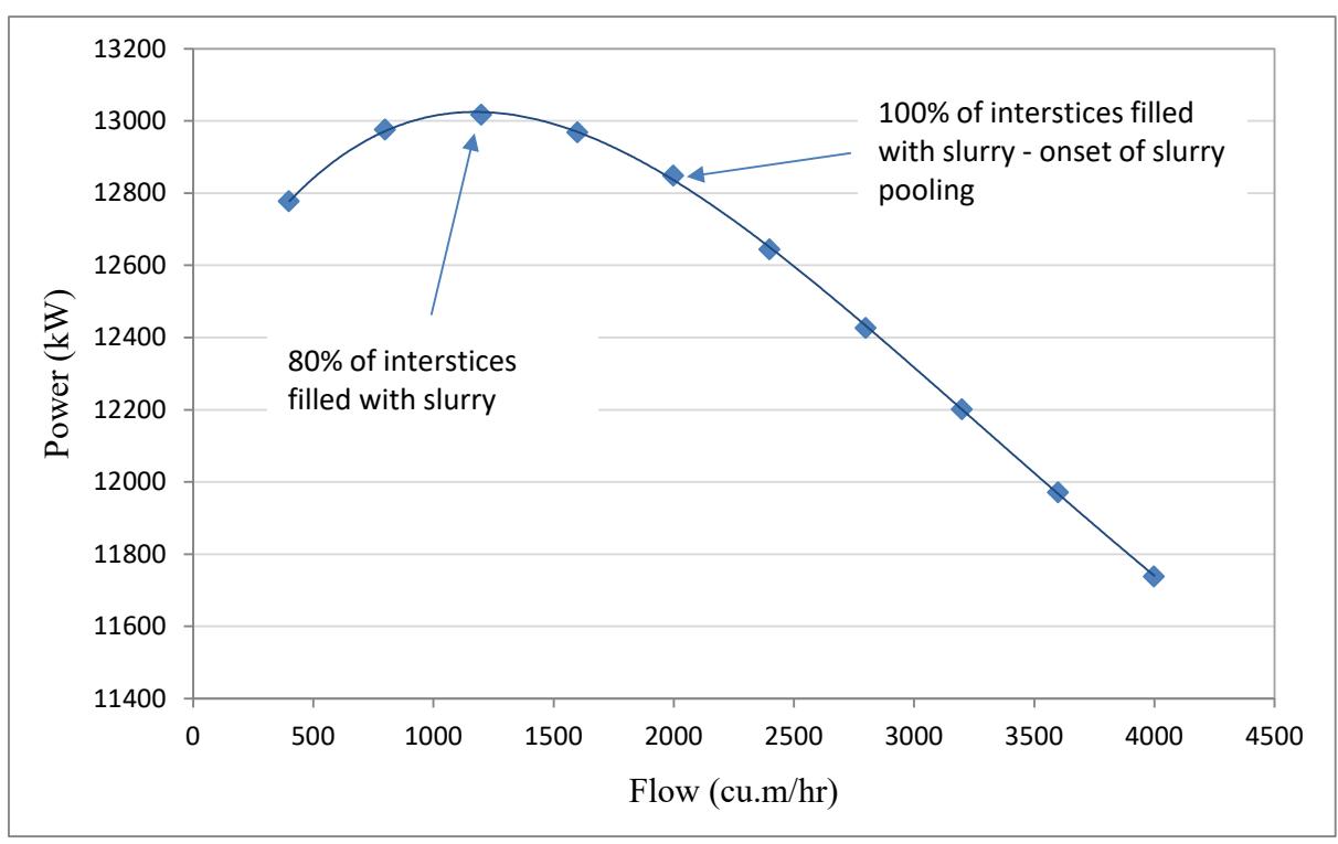
As the mill was operating under slurry pool conditions, increasing flowrate decreased power draw. If the mill did not have a slurry pool in the first instance this response may not have occurred. Figure 13 shows the predicted full range of power response to changes in flowrate. As can be seen it is parabolic in nature with maximum power draw being drawn when the media interstices are about 80% full of slurry. The implications of this response is that if the mill is operating to the left of the maximum, increasing flow rate will cause the power draw to increase. However if the mill is operating to the right of the maximum, exactly the opposite response will result.
3.3 Predicting θ tp in Overflow Discharge Mills
An overflow mill can be considered as a special case of a grate discharge mill in which the grates have no holes (or all of the holes are blocked) and slurry builds up until it overflows out of the discharge trunnion. At this point θtp is referred to as the slurry overflow angle θto. From a power draw modelling viewpoint the position of the slurry pool, as measured by the toe angle θto, can be calculated theoretically from a knowledge of the trunnion diameter, mill diameter and slurry level within the mill.
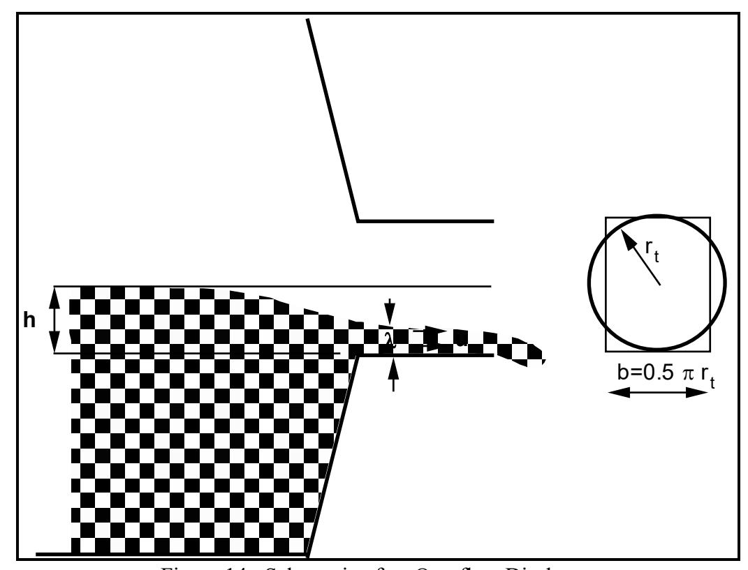
The slurry level will vary with flow of slurry into and out of the mill, a higher level resulting from a higher flow. The slurry level can be estimated by making the simplifying assumption that the discharge trunnion behaves like a rectangular section, broad crested weir (Figure 14).
By applying the Bernoulli equation to such a weir of width b, then the velocity (u) at the end of the weir can be obtained by solving:
The volumetric discharge rate (Q) is therefore given by:
$$ Q = b\lambda(2g)^{0.5} (h-\lambda)^{0.5} $$ (10)
For maximum discharge
$$ \frac{dQ}{d\lambda} $$ = 0 at constant h
By differentiating equation 10 and setting \( dQ/d\lambda \) to zero gives:
By substituting for \( \lambda \) in equation 10 therefore gives:
To maintain the same cross-sectional area and maximum vertical height as the mill discharge trunnion, b must be set to \( \pi r_t/2 \)
Hence $$ Q_{\text{max}} = 0.5 \, \pi r_t \, g^{0.5} \, (0.67h)^{1.5} $$ (12)
or h = $$ 0.67 \left( \frac{2Q}{\pi r_t g^{0.5}} \right)^{2/3} $$ (13)
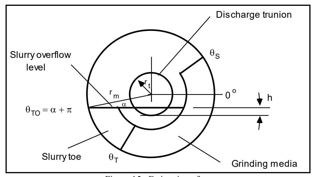
With reference to Figure 15, \( \theta_{to} \) can be calculated as follows:
$$ \theta_{to} = \arcsin\left(\frac{r_t - h}{r_m}\right) + \pi $$ (14)
By substituting equation 13 into equation 14, \( \theta_{to} \) can be found.
These equations are theoretical and relate to inviscid flow. In practice slurries are far from inviscid in behaviour. Empirical corrections to equation 13 are necessary to reflect slurry behaviour. In practice this will result in the distance, h, being higher for a given slurry flow than equation 13 suggests. To account for this a multiplier is applied to equation 13. On the basis of operating data collected so far, this multiplier is of the order of 2.
The validity of these equations is illustrated using the data from Figure 5 which is reproduced in Figure 16 with Citic SMCC's model predictions overlaid. Good agreement is seen.
4. Conclusions
The behaviour of the slurry phase in tumbling mills influences their power draw. Whereas in some instances this influence is relatively minor, in other cases it can be profound. For a power model to be truly effective, therefore, this response must be adequately described. Citic SMCC's power does so by describing the power draw of the slurry phase separately to the grinding media, then adds the values to give the overall power. This is in contrast to other published models which do not consider the slurry phase at all.
The volume occupied by the slurry phase is dictated by the design of the discharge system, the volume of grinding media and the slurry flowrate. The Citic SMCC model utilises equations which initially predict the volume of the slurry phase then uses this information to predict its position and motion in relation to the grinding media phase.
The model has been tested using a large volume of operational data and has been demonstrated to provide very accurate results.
5. Reference
Arbiter N. and Harris C.C., 1982. Scale-up and Dynamics of Large Grinding Mills - a Case Study. Design and Installation of Comminution Circuits, Mular A.L. and Jergensen II.G.V. (eds) AIME, New York, Ch 26, pp 491-505.
Austin L.G., 1990. A mill power equation for SAG mills. Minerals and Metallurgical Processing. pp 57 - 63.
Bond F.C. 1961. Crushing and Grinding Calculations Part I and II. British Chem Eng 6(6) 378-385
Hogg R. and Fuerstenau D.W., 1972. Power relationships for tumbling mills. Trans. SME/AIME, 252, pp 418 - 423.
Latchireddi, S R., 2002. Modelling the performance of grates and pulp lifters in autogenous and semi-autogenous mills. PhD thesis. University of Queensland. Australia.
Latchireddi, S. and Morrell, S. (2003a). Slurry flow in mills: grate-only discharge mechanism (Part1). Minerals Engineering, Volume 16, Issue 7, July, Pages 625-633.
Latchireddi, S. and Morrell, S. (2003b). Slurry flow in mills: grate-pulp lifter discharge systems (Part 2). Minerals Engineering, Volume 16, Issue 7, July, Pages 635-642.
Morrell, S., 1989. Simulation of bauxite grinding in a semi-autogenous mill and DSM screen circuit. M.Eng thesis. University of Queensland. Australia
Morrell, S. and Latchireddi, S. (2000). The operation and interaction of grates and pulp lifters in autogenous and semi-autogenous mills. Seventh Mill Operator's Conference, Kalgoorlie, WA., pp 13-19, AusIMM.
Morrell, S and Stephenson, I., 1996. Slurry discharge capacity of autogenous and semiautogenous mills and the effect of grate design. Int. J. Miner. Process, 46(1-2) : 53.
Morrell, S. (1992). Prediction of grinding mill power. Trans Inst Min Metall, Section C Vol 101 (C1-60): 25-32
Morrell, S., 1993. The prediction of power draw in wet tumbling mills. PhD thesis. University of Queensland. Australia
Morrell, S. 1996a. Power draw of wet tumbling mills and its relationship to charge dynamics - Part 1: a continuum approach to mathematical modelling of mill power draw. Trans Inst Min Metall, Section C Vol 105, C43-53.
Morrell, S and Kojovic, T., 1996. The influence of slurry transport on the power draw of autogenous and semi-autogenous mills, Proc. Of 2nd Int. Conf. on Autogenous and Semiautogenous Grinding Technology, Vancouver, Canada., pp.378-389.
Napier-Munn, T. J., Morrell, S., Morrison, R. D. and Kojovic, T., 1996. Mineral Comminution Circuits Their Operation and Optimisation, JKMRC Monograph Series 2, pp 247-272.