ORE CHARGE, BALL LOAD AND MATERIAL FLOW EFFECTS ON AN ENERGY BASED SAG MILL MODEL

S. MORRELL¹ and R. D. MORRISON^{2 1}Julius Kruttschnitt Mineral Research Centre ²JK Tech, Commercial Division, Julius Kruttschnitt Mineral Research Centre

SUMMARY

Techniques have been developed at the Julius Kruttschnitt Mineral Research Centre which relate energy to corresponding breakage in laboratory scale tests. These relationships can be applied to autogenous mill modelling.

For each ore type, specific breakage distributions are measured for both high energy (impact or crushing) and low energy (abrasion) breakage. Energy levels in the mill are estimated, for each particle size range, from the mill load (determined recursively) and mill size. Combining these gives breakage (appearance) distribution functions for the mill. Transport through the mill is determined by the grate size and pebble port size modelled as a classification function. An empirical mass transfer function is used to relate the holdup of fine material in the mill to the mill feed rate. The perfect mixing matrix comminution model is used to calculate mill discharge and contents. For semi-autogenous grinding the ball load is converted to an equivalent additional ore load to allow the energy levels to be calculated.

As the JKMRC SAG/Auto mill data base expands, various mass transfer relationships have been tested against real data. This paper presents a transfer function based on a wide range of data. The effect of ball load has been investigated for a range of ore types. These data suggest a systematic relationship between ball load and grinding rates. This relationship is presented and discussed.

INTRODUCTION

The JKMRC has been concerned with modelling of autogenous and semiautogenous mills since the early 1970s (Stanley, Gault, Duckworth). A large number of these mills have been investigated. The key problem which arose was to separate the breakage process from the others occurring within the mill and to quantify this process in terms of the grinding media, that is, the mill load. This paper outlines the modelling approach developed by Leung (1987) and subsequent developments concerning the effects of ball load and the factors governing the flow of material through the mill.

INPUT ENERGY - BREAKAGE MODELLING

Early researchers into grinding were concerned with the energy consumed by specific process units for size reduction of various ore types. Since the late 1970s the JKMRC has been investigating single particle breakage under closely controlled conditions to separate process unit effects (i.e. type of mill) from the specific breakage behaviour of a particular ore.

The early definitions of breakage functions arose from the work of Broadbent and Calcott (Lynch, 1977, Chapter 2) - dropping lumps of coal onto hard surfaces.

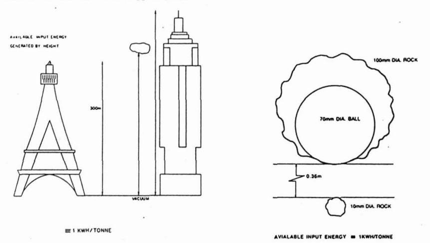
It is difficult to achieve industrial energy levels by dropping lumps of ore. Achieving even one kilowatt hour per ton of energy input requires a vertical drop of more than 300m. A more realistic (and less hazardous) experimental technique is to hit small rocks with larger ones (Figure 1). Assuming the small particle absorbs all the energy, then a drop of 360mm by a 100mm diameter particle onto a 10mm diameter particle achieves the same energy input. If the ore has a specific gravity of around 2.67, then a 70mm diameter steel ball achieves the same energy input.

PENDULUM TEST WORK

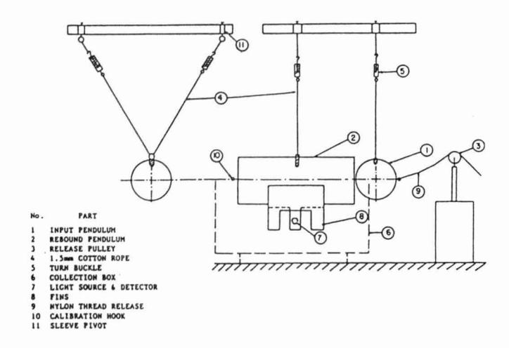
Researchers (Narayanan and Whiten, 1983) at the JKMRC have investigated breakage using a modified ballistic pendulum. The rebound pendulum is instrumented, as shown in Figure 2, to allow the absorbed energy to be monitored from the amplitude of the pendulum. A computer is used to measure the time between fins interrupting a transverse laser beam. The input pendulum can be released from controlled heights for precise control of input energy. 25-100 particles are broken one at a time in several closely controlled size and input energy ranges. It turns out that the degree of breakage can be usefully described by the percentage of the original particle which passes through an aperture of one tenth of the original particle size.

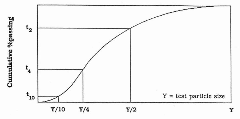
This percentage is called the \( t_{10} \) and was found to be simply related to the specific crushing energy in the following way:

$$ t_{10} = a(1 - e^{bE_{cs}}) $$ where $$ a,b = constants $$ specific crushing energy

It has also been found that the relationship between the \( t_{10} \) and other points on the size distribution depends only on the value of \( t_{10} \) for a wide range of ore types. Graphically, this is shown in Figures 3 and 4.

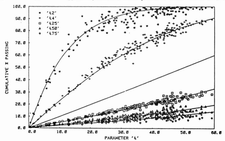
The relationships depicted in Figure 4 can also be described mathematically in the following manner (Leung 1987):

$$ P = 1 - (1 - x)^{e^g(-\ln(1-t))^A} $$ (2) where $$ A = 1 + 0.0898 \ln(10x) - 0.429 (x - 0.1) $$ g = 0.88 \( \ln(10x) e^{0.672x} - \ln(-\ln(1-t)) \) and $$ P = \text{cumulative fraction passing } x = \text{normalised size } t = \text{cumulative fraction passing } x = 0.1(t_{10}) $$

Hence if an energy level for a particular particle size is known a \( t_{10} \) can be calculated to reconstruct the complete size distribution or appearance function.

AUTOGENOUS MILL BREAKAGE

To provide an initial energy level, Leung (1987) assumed that the energy levels for the coarsest size fractions of the mill load could be scaled against the mill diameter, that is, the maximum particle lift should be proportional to mill diameter.

$$ E_1 = \rho * g * mill diameter $$ (3)

For the smaller sizes Leung followed a functional form proposed by Austin et al. (1984).

This assumes that each size fraction within a mill load will experience a different input energy level and will, therefore, produce a different breakage function.

BREAKAGE BY ABRASION

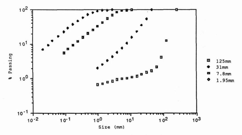
Each of the earlier researchers had identified a proportion of fine particles which were produced by chipping off the sharp edges. Leung (1987) generated abrasion or low energy appearance functions from tumbling tests in the laboratory under a standard set of conditions. Using an approach similar to that of Narayanan and Whiten (1983) in their work on impact breakage he developed an ore specific t parameter for abrasion. This is used to generate an appearance function which is combined with that for impact to produce a combined appearance function as shown below. Figure 5 shows typical combined appearance functions for a range of sizes.

$$ a = \frac{t_{LE} a_{LE} + t_{HE} a_{HE}}{t_{LE} + t_{HE}} $$ (5)

where

a = combined appearance function tLE = t parameter for abrasion tHE = t parameter for impact breakage aLE = abrasion appearance function aHE = crushing appearance function

MODEL STRUCTURE

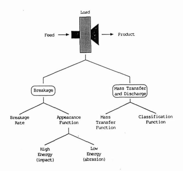
The perfect mixing mill model (Whiten, 1974) at steady state provides the structure to combine the ore specific breakage function with the other components of the model shown in Figure 6. The model is arranged to predict mill load as well as mill product. It relates the different parts in the following manner.

$$ f_i - d_i s_i + \sum_{j=1}^{j-1} r_j s_j a_{ij} - (1 - a_{ii}) r_{ii} s_i = 0 $$ (6)

$$ p_i = d_i * s_i $$ (7)

where \( f_i \) , \( s_i \) , \( r_i \) , \( d_i \) and \( p_i \) are feed rate, contents, breakage rates, discharge rates and product rate vectors and \( a_{ij} \) is the combined appearance or breakage distribution function. The size fraction indices ( i or j) count from the coarsest screen size to the finest. The form of equations (6) and (7) allows both the mill load and the product to be calculated from a mill feed and a set of breakage and discharge rates.

BREAKAGE RATES

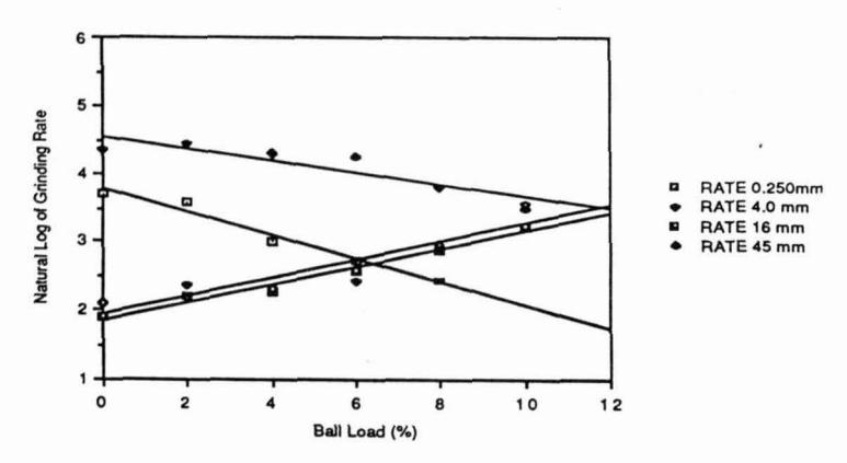
The Leung (1987) approach was to propose that for any load environment, the grinding rates will be constant - at least to a first approximation. Clearly where balls are a significant proportion of the load, they will not break or abrade and the grinding rates must change. Leung approximated the energy input of the balls by converting them to an equivalent load of the same specific gravity as the ore itself. A steel ball is assumed to provide equivalent energy input to an ore particle of the same mass.

Most of the data available to Leung was either autogeneous or close to a 6% ball charge. Hence a set of average rates could be derived for each of these conditions. As shown in equation 6, the model utilises a grinding rate r₁ for each size fraction. As there may be up to thirty square root of two size fractions in a mill feed, these rates are compacted into a spline function (Ahlberg, 1967) with five knots. A spline function is a smooth curve with a continuous first derivative and a second derivative which may change at each knot. The curve is equivalent to a draftsman's spline - a strip of steel adjustable by moveable screws. The screw positions are analagous to the knot positions. With the expanding use of JKSimMet and continuing research (Morrell 1989), a much broader range of data is becoming available.

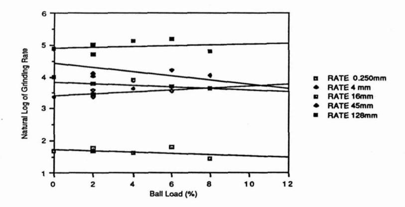
These data include several 1.8m \( \times \) 0.6m mill pilot tests with 2% increments in ball charge.

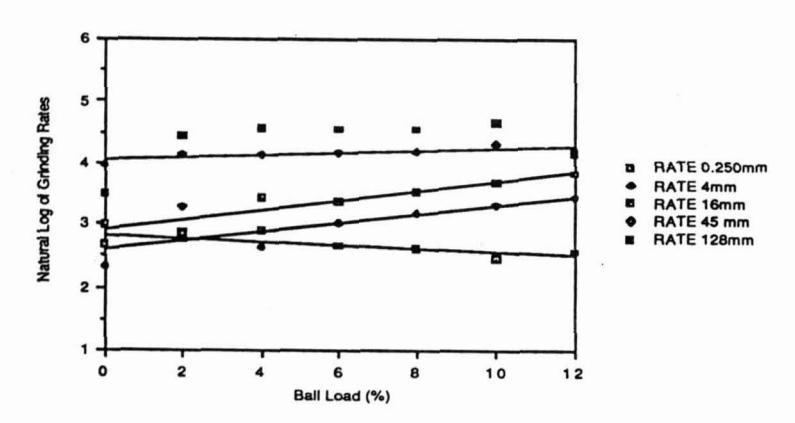
These data are not available for general publication, however the grinding rates at each spline knot are shown in Figures 7, 8 and 9 for three ores of varying hardness.

The rates reported also cover a range of circuit configurations from open circuit to closed with one or two stages of classification.

While some variation in the rates is apparent for different ore types, in each case, the variation with ball charge is quite systematic.

Some of these data also include large variations in the ball size distribution.

MASS TRANSFER

To calculate the mill load we require knowledge of how much minus grate size material will remain in the mill with different operating conditions. In the absence of a more realistic relationship at that time, Leung (1987) adopted the simple model proposed by Austin et al (1976). This took the following form:

$$ L = m_1 F^{m_2} $$ (8)

where

\( m_1, m_2 = constants \)

= fraction of the mill volume occupied by below grate size ore and water

F = volumetric discharge rate expressed as equivalent mills full per minute

Using his own experimental results from tests conducted with a 1.73m diameter mill and augmented by the results of Stanley's work on the Warrego mill (1974) Leung estimated the values of \( m_1 \) and \( m_2 \) to be both equal to 0.37.

Since then Rogers and Austin (1984) and Moys (1985) have proposed more comprehensive relationships which incorporate a range of mill and slurry variables. One of the major problems with these, or any other relationships relating to SAG/FAG mills, has been in obtaining data to verify and refine them.

JKMRC SAG MILL DATA BASE

As noted earlier, the JKMRC SAG/FAG mill data base has been considerably expanded through the contribution of detailed pilot mill results from several sources and data from the Alcoa of Australia Pinjarra SAG mills. The data from Alcoa were obtained during a two year SAG mill study sponsored by Alcoa and undertaken by the JKMRC. As part of the project an entire equilibrium charge from one of their 7.3m diameter mills was dropped, weighed and sized. It is believed that this is only the second time that this has been done in Australia, the first being Stanley's analysis of the Warrego mill charge (1974).

The JKMRC SAG mill data base now includes results from 43 tests for which full circuit surveys and mill charge size distributions are available. Of these, two are from industrial scale mills with the remainder being from pilot scale mills with diameters of the order of 1.8m. This has now put us in a position to draw tentative conclusions about the effects not only of operating conditions but mill design factors as well.

FACTORS AFFECTING THE MASS TRANSFER RATE

A list of potentially significant variables can be drawn up as follows:

Mill variables: diameter

length

grate open area grate design speed

shape

Ore/charge variables: charge porosity

pulp level pulp s.g. pulp viscosity

charge flow characteristic

With the exception of mill shape and the ore charge flow characteristic the above variables are self explanatory. Mill shape and grate design have been included for the sake of completeness though they have not been included in this analysis. The former is a term which covers such design features as liner profile and the degree to which the mill ends are conical in shape. The grate design term relates to the hole positioning and whether round, square or slotted apertures are used. The flow characteristic will be considered later and describes how well a charge flows.

FORMULATION OF AN EMPIRICAL MASS TRANSFER RELATIONSHIP

Using the JKMRC data base, multiple regression techniques were applied to derive an empirical relationship between the volumetric discharge rate and operating and design variables. The following equation was obtained:

$$ Q = K \phi_c^a E^b \lambda^c L_p^d A^e D^f $$ (9)

where K, a, b, c, d, e, f фс fractional critical speed Eλ porosity factor 1.0 - recycle fraction fractional mill pulp filling A open area of grate (m2) D mill diameter (m) volumetric discharge rate 0 (m³/min)

Values for the constants were as follows:

K = 0.001 a = 9.37 b = 1.327 c = -0.805 d = 0.249 e = 0.952 f = 3.264

Only coefficients which were significant at the 95% level were included. The \( \rm R^2 \) value was 0.977 which is significant at the 99.99% level. Figure 10 shows a plot of the observed discharge rates and those predicted by equation 9.

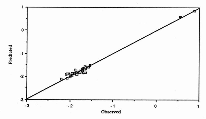
The inclusion of the one minus recycle fraction term is particularly interesting. The recycle fraction is defined as the fraction of total feed to the mill which has been recycled by the circuit classifier. In the case of open circuit operation the recycle fraction is zero and the term has a value of unity. It is suggested that the recycle fraction reflects the flow characteristic of the mill feed and hence mill charge. By definition recycled material is able to flow through the mill and therefore it is not unreasonable to expect that the higher is its proportion in the mill feed the higher will be the discharge rate. The ability of the recycled material to flow through the mill will obviously be related to its size though the shape also is likely to play an important role as it will be typically be smooth and well rounded.

The porosity factor indicates the ability of a coarser charge to allow pulp to flow through it more easily. It is not a true porosity but an indication of it using the following definition:

$$ E = \% $$ charge > 4 * grate aperture (10)

The other terms in equation (9) indicate that higher discharge rates will result if the mill diameter, grate open area, mill speed or mill pulp level are increased.

Interestingly the pulp s.g. was not found to be a significant variable. However, Stanley's (1974) results indicate that as the percent solids increases the level of pulp within the mill rises in an attempt to maintain the discharge rate. This effect is probably due to the resultant increase in viscosity rather than an s.g. effect per se. Work at the Alcoa Pinjarra refinery (Morrell, 1989) has shown that the pulp viscosity has a considerable influence on the performance of the milling and classification circuits and its exclusion from equations describing them results in a much weaker relationship between their performance and operating variables. The viscosity - s.g. relationship, however, varies from one ore type to another and therefore will not be consistent in the JKMRC data base. Unfortunately, viscosities are only available for the Alcoa data set and therefore at this stage its effect and that of the pulp s.g. cannot be enumerated.

DISCHARGE FUNCTION

Given a defined and perfectly mixed mill load, we can calculate a product if we know a discharge rate for all size fractions. The discharge rate is considered to be the product of two mechanisms, viz. transport to and classification by the grate. Clearly,

• \( ^{\bullet} \) above the grate size \( (x_q) \) , the discharge rate will be zero
• * below a certain size \( (x_m) \) , the pulp will behave "like water" and the discharge rate will be at a constant maximum.
• between the sizes \( x_m \) and \( x_g \) the discharge rate will be dependent upon the classification behaviour of the grate. The grate classification function used in the model is as follows:

$$ C_{i} = \frac{\ln (x_{i}) - \ln (x_{g})}{\ln (x_{m}) - \ln (x_{g})} ; x_{g} > x_{i} > x_{m} $$ (11)

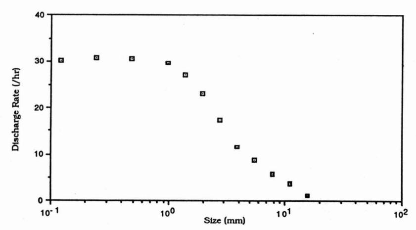
The discharge rate for a specific size fraction is therefore the product of the classification function for that size and the maximum discharge rate, ie, the discharge rate for sizes less than xm..

If the mill contents are sampled, the shape of the discharge function can be easily calculated. Figure 11 shows the discharge function from Alcoa's mill.

MODEL OPERATION

The model adjusts the overall discharge rate until it operates on the mass transfer line. That is, if the retention of minus grate size material is above the line, the discharge rate is increased and vice versa.

CONCLUSIONS

The Leung model (1987) is finding increasing use in industry through the JKSimMet package. Approximately 50 of these systems are in use world wide. The Leung model has proved to be an excellent description

of both full scale and pilot scale autogenous and SAG mills. The effects of ball charge on grinding rates are quite systematic but do vary in magnitude for different ore types and different ball size distributions.

Through the use of the JKMRC FAG/SAG mill data base tentative conclusions can now be drawn on the relative effects of operating and design variables on the mass transfer rate. First indications have shown that factors such as the charge porosity and the recycle load significantly affect the flow of material through the mill.

The model can be used to interpolate between measured operating conditions and to provide estimates for variations in:

ball load ball sizings feed sizings grate size

and in circuit configuration with other comminution or classification devices.

Hence it provides a powerful tool for:

• optimisation of existing circuit
• exploring design options (as an enhancement to traditional design techniques)
• a first pass grinding circuit design on the basis of small samples - even drill cores.

FUTURE WORK

The scale up properties of any model can only be reallistically assessed in a genuine design situation. The Leung model has now been used in several SAG mill designs in Australia. These plants are now starting to come on stream. We are currently carrying out audits at two of these plants. Some results should be available for presentation in September.

General development of the Leung model is proceeding at the JKMRC with the objective of improving grinding rate and discharge rate predictions over a wider range of mill types and operating conditions.

ACKNOWLEDGEMENTS

The contributions of Alcoa of Australia and the sponsors of the AMIRA mineral processing project are gratefully acknowledged.

REFERENCES

AHLBERG, J.H., NILSON, E.N.and WALSH, J.L., 1967, "The Theory of Splines and Their Applications", Mathematics in Science and Engineering, Volume 38, Academic Press, New York and London.

AUSTIN, L. G., LUCKIE, P.T. and KLIMPEL, R.R., 1984, "The process engineering of size reduction: Ball Milling", S.M.E./A.I.M.E., New York, 561pp.

AUSTIN, L.G., WEYMONT, N.P., PRISBREY, K.A., and HOOVER, M., 1976, "Preliminary Results on the Modeling of Autogenous Grinding", Proceedings of the 14th International APCOM Conference, The Pensylvania State University, New York, October, pp 207-226

DUCKWORTH, C. A. and LYNCH, A.J., 1982, "The effect of some operating variables on autogenous grinding circuits and their implications for control", C.I.M. XIV Int.ernational Mineral Processing Congress, Toronto.

GAULT, G.A., 1975, "Modelling and control of autogenous grinding circuits" PhD Thesis (unpublished), University of Queensland, Australia.

LEUNG, K., 1987, "An energy based ore specific model for autogenous and semi-autogenous grinding" PhD Thesis (unpublished), University of Queensland.

LEUNG, K., MORRISON, R.D. and WHITEN, W. J., 1987, "An energy based ore specific model for autogenous and semi-autogenous grinding" Copper 87, Santiago, Chile.

LYNCH, A. J., 1977, Mineral Crushing and Grinding Circuits, Elsevier Scientific Publishing Company, Amsterdam: 340pp.

MORRELL, S., 1989, "Simulation of Bauxite Grinding in a Semi-Autogenous Mill and DSM Screen Circuit", ME Thesis (in preparation), University of Queensland.

MOYS, M.H., 1986, "The Effect of Grate Design on the Behaviour of Grate-Discharge Grinding Mills", International Journal of Mineral Processing, 18, pp. 85-105.

NARAYANAN, S.S. and WHITEN, W.J., 1983, "Breakage characteristics of ores for ball mill modelling", Proceedings Australasian Institute Min.ng and Metall.urgy, No. 286, June: 31-30pp.

ROGERS, R.S.C. and AUSTIN, L.G., 1984, "Residence Time Distributions in Ball Mills", Particulate Science and Technology, Vol. 2, 2, pp. 191-209.

STANLEY, G.G., 1974, "Mechanisms in the autogenous mill and their mathematical representation", Journal of the South African Institute of Mining and Metallurgy, Nov: 77-98pp.

WHITEN, W.J., 1974, "A matrix theory of comminution machines", Chemical Engineering Science, No. 29, 588-599pp.