



The content on this page was automatically generated from the PDF publication document and may contain errors or inaccuracies. Please refer to the original PDF for the most accurate information.
OVERALL SPECIFIC ENERGY REQUIREMENT OF CRUSHING, HIGH PRESSURE GRINDING ROLL AND TUMBLING MILL CIRCUITS
1 BACKGROUND
20 years ago discussions about conventional comminution circuits would revolve around crushing-rod-ball or crushing-ball circuits and the work of Bond (1961) would provide the principal tools in determining what the specific energy of the associated circuits should be. Nowadays, such circuits are all but obsolete and are mainly confined to relatively small operations. Autogenous (AG) and Semi-autogenous (SAG) milling, often combined with ball milling, now dominate comminution circuit configurations with strong signs that High Pressure Grinding Rolls (HPGR) are poised to make major inroads as alternatives to AG and SAG mills in some applications. Bond's specific energy equations and rock characterisation techniques were not originally designed for such circuits and though a number of people have tried to apply them over the years to AG and SAG circuits they have not always been found to be reliable. In the case of HPGR circuits Bond's methodologies are completely inappropriate. Despite this, the underlying principle of predicting the specific energy of a comminution circuit then using this in conjunction with the required throughput to obtain the associated power demand is still the approach adopted today in the design of comminution circuits. The question then is: what equations can be used for modern comminution circuits if Bond's published equations are increasingly irrelevant? This chapter seeks to answer this question.
2 ENERGY-SIZE RELATIONSHIPS
2.1 General
It has been 60 years since Bond (1952) published his theory of comminution and over 125 years since von Rittinger (1867) and Kick (1885) published theirs. All of them relate size reduction and material properties to specific energy (so called Energy-Size Relationships) As pointed out by Hukki (1961) all of the equations that these researchers developed are special forms of the same differential equation as proposed by Walker et. al. (1937). This equation can be written as:
where
E = net energy required per unit weight (specific energy)
x = index describing the size distribution, eg p80
n = exponent indicating the order of the process
C = constant related to material properties and the units chosen to balance the equation
If the exponent in equation 1 is set to values 2, 1.5 and 1 then integrated, the equations proposed by von Rittinger, Bond and Kick respectively are obtained:
where
\( E_{1-2} \) = Net specific energy to reduce size distribution 1 to distribution 2
\( x_1, x_2 \) = Size distribution indices where \( x_1 > x_2 \)
Hukki's evaluation of these equations led him to conclude that each might well be applicable but only in a relatively narrow size distribution range. He further postulated that the equation of Walker et al had the wrong form and that the exponent, n, was not constant but varied with the magnitude of the size distribution index, x. He therefore suggested that a more appropriate general differential equation was:
Hukki did not specify what the function f(x) was, though he described experiments that might provide data to determine what it should be. Despite the conclusions of Hukki concerning the limitations of Bond's equation, since its publication it has become the industry standard for estimating the comminution energy required to reduce rock from one size to another and has been applied to all comminution steps (rightly or wrongly) ranging from blasting to fine grinding. Various factors have been added, depending on the application, with the intention of improving its accuracy. However, the basic equation, in which energy is related to the inverse square root of particle size has remained unchanged. The question therefore still remains as to whether this is valid over the full range of particle sizes reduced in comminution circuits and whether an alternative approach is more suitable. This is particularly relevant to autogenous (AG), semi-autogenous (SAG) and ball mills, which currently are by far the most popular choice for grinding circuits in the gold and base metal sectors.
2.2 Bond's Equations
Bond's so-called "Third Theory" equation is normally written as:
where
W = Specific energy
Wi = Work index
P = 80% passing size for the product
F = 80% passing size for the feed
The work index \( (W_i) \) was defined by Bond as the "....comminution parameter which expresses the resistance of the material to crushing and grinding". In practice \( W_i \) has to be determined from plant data or by conducting grinding tests in which W, P and F are measured. If plant data are available equation 6 is rearranged, the work index being referred to as the operating work index \( (OW_i) \) :
Where plant data are not available the work index has to be determined from laboratory milling tests. Bond developed rod and ball mill laboratory tests for this purpose. The work indices that they produce are in effect operating work indices and are calculated using feed and product sizes using standard test conditions. It was assumed by Bond that the net energy consumption per revolution of the test mills he used remained constant. Levin (1989) estimates that on average this value is 198.4 kWh/rev x 10-7, but states it is far from constant. This value was implicitly incorporated by Bond (1962) in his equation for determining the laboratory ball mill work index, by calibrating his laboratory procedure with full scale mill data. The equation he developed to estimate the ball mill work index using his laboratory test mill is:
$$ W_{i} = \frac{49}{P_{1}^{0.23} (Gbp)^{0.82} 10 \left(\frac{1}{\sqrt{P}} - \frac{1}{\sqrt{F}}\right)} $$ (8)
where
Wi = Bond laboratory ball work index (kWh/tonne)
\( P_1 \) = closing screen size in microns
Gbp = net grams of screen undersize per mill revolution
P = 80% passing size of the product in microns
F = 80% passing size of the feed in microns
Bond also developed laboratory rod mill and crushing tests, each with its own (different) equation for determining the work index. He recommended that the laboratory tests were carried out so that they generated a similar product size to the proposed full scale circuit. Thus any errors associated with an incorrect exponent were minimised, as the Bond laboratory test procedure and his equation for predicting full-scale performance have the same (incorrect) exponent. This can be shown mathematically by combining equations 6 and 8 and assuming that the laboratory test feed and product are the same as the full-scale plant. The full scale specific energy (W) is given by the expression:
When the conditions proposed for the full-scale plant begin to depart significantly from those of the laboratory test, the Bond equation becomes progressively inaccurate. However, Bond introduced a number of correction factors for such situations and these have been expanded and modified over the years (Rowland and Kjos (1980)) in an attempt to cater for changing circuit designs, in particular the introduction of AG and SAG mills (Barratt and Allan (1986)). As a result there are a number of "rules", mostly unpublished, which are applied by comminution circuit designers to make Bond's equations more applicable to these circuits. This is a most unsatisfactory situation as it does not address the fundamental problem with the equation, merely attempts to treat the symptoms of its inadequacy.
2.3 Validity of Bond's Equations
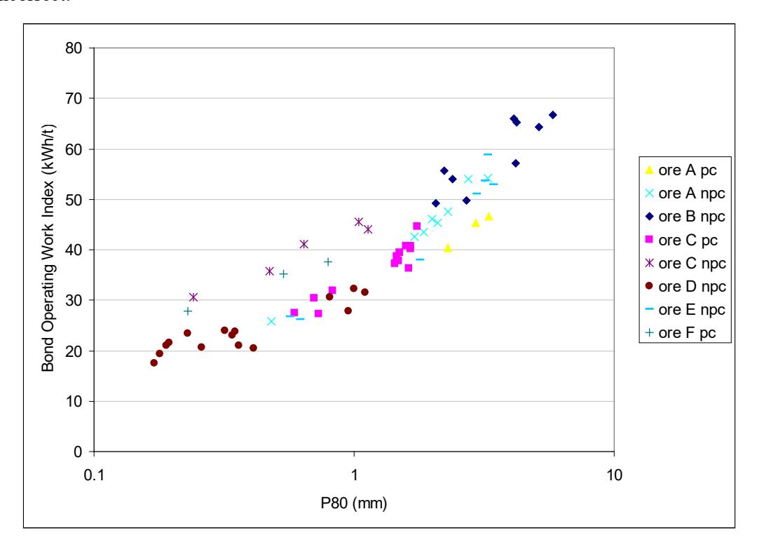
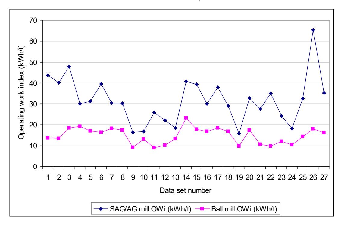
If Bond's equation holds, then for a given comminution step, regardless of the feed and product size, the Bond operating work index (OWi) should remain constant. This should be true providing the efficiency of the comminution step remains constant as well as the resistance to breakage of the rock. Data from different pilot AG/SAG mill programmes were analysed using equation 7 to see whether the Bond OWi did indeed remain constant regardless of the feed f80 and product p80 sizes. The data comprise 8 different programmes using 6 different ore types. The individual results in each programme represent tests run with different ball charges, closing screen sizes and feed sizes. The results are summarised in Figure 1. In all of the 8 programmes the Bond OWi was not found to be constant but decreased as the product size became finer, indicating a systematic bias in Bond's equation. Further evidence of this trend was found in the differences between the Bond OWi for AG/SAG mills and the ball mills that they feed. This is illustrated in Figure 2 where the Bond operating work indices from 27 full scale AG/SAG – ball mill data sets are presented. In each case the data sets comprised a feed size, product size and specific energy for both the AG/SAG mill and ball mill circuits, the product size of the AG/SAG mill circuit being the feed to the ball mill circuit. All of the work indices from the AG/SAG circuits were found to be significantly higher than their associated ball mill data, on average being 115% higher.
It is possible that these results could reflect differences in the efficiency of AG/SAG mills compared to ball mills ie ball mills are more efficient than AG/SAG mills. However, a study by Morrell et al (1991) of a SAG-ball mill circuit running in parallel with a multi-stage ball mill circuit crushing and grinding the same feed to the same product size showed that the specific energy for each circuit was identical, ie they had the same energy efficiency. Further evidence of this was reported by Larsen et al (2001) from pilot studies of various circuit configurations. These included single stage AG/SAG milling, AG/SAG milling followed by ball/pebble milling and rod/ball milling. They concluded that, regardless of how the circuit was configured, the overall power consumption remained the same within the limits of data accuracy ie the energy efficiency of AG/SAG mills and ball mills was similar. This is not to say that all circuits, regardless of how they are operated, will have the same energy efficiency. It is not very difficult to operate a circuit in a way that will significantly affect its energy efficiency eg poor classification, incorrect ball size, inappropriate slurry density can increase significantly the specific energy required to grind to a specified product size. However, it is asserted that in most cases, providing circuits are operated under optimum conditions, the overall specific energy to grind a particular ore from a specified feed f80 to a specified product p80 will be similar, at least to within +/- 5%, regardless of the circuit configuration.
Another interpretation of the data in Figures 1 and 2 might be that the changes in operating work index reflect changes in the resistance to breakage as the product size varies. However, research has shown that the resistance to breakage tends to increase as particle size reduces
(Tavares and King (1998)), whereas the data in Figures 1 and 2 would suggest the opposite. It is concluded that the most likely reason for these trends is that the Bond equation is incorrect.
3 AN ALTERNATIVE ENERGY-SIZE RELATIONSHIP
3.1 General
The trend of increasing Bond operating work index as product size increases, points to a relationship such as that proposed by Hukki as being more appropriate. However, Hukki's equation, as with Walker's, assumes constant material properties with respect to particle size. As previously stated this has been shown to be incorrect, rock strength typically increasing as size decreases. This phenomenon is attributed to the size and density of pre-existing cracks and imperfections, which reduce as particle size reduces (Griffith (1920), Weibull (1939), Rumpf (1973)). Further evidence of this phenomenon is sometimes inferred from Bond laboratory tests at different closing screen sizes. These results sometimes show a trend of increasing laboratory work index as the closing screen size decreases (Blaskett, 1969). However, it is dangerous to draw these conclusions from the Bond laboratory test as the equation for determining the work index (eq. 8) tends to naturally generate such trends due to the inclusion of the closing screen size in the denominator.
It has been proposed (Morrell, 2004) that a more complete description of a general form of comminution equation is given by:
where
g(x) = function describing the variation in breakage properties with particle size
C = constant related to the breakage properties of the material
From a practical viewpoint one of the problems with equation 10 is that the variation in breakage properties with particle size is not the same for all rocks (Morrell et al (2001)). Hence there is unlikely to be a function g(x) that will satisfy all rock types, though there is evidence that some rocks behave in a broadly similar manner. A general solution to the equation is therefore unlikely to be found. In addition, the experimental determination of the size-by-size properties of a rock over the typical range of feed f80 sizes handled in a comminution circuit (-150mm+0.045mm) would be very difficult, a problem further complicated by the lack of a proven procedure for carrying out such experiments. Practically, therefore, there is little recourse at the current time but to use a value for the breakage property of an ore that does not vary with particle size.
3.2 Energy-Size Equation
Given this situation, a practical solution in the form of an equation that relates specific energy to size reduction is given below (Morrell, 2004). The rock breakage properties, as represented by a comminution index \( M_i \) , are assumed to be constant with respect to particle size, leaving any variation to be taken up in the form of the function f(x).
where
W = Specific energy (kWh/tonne)
K = Constant chosen to balance the units of the equation
\( M_i \) = Index related to how an ore breaks in the comminution device (kWh/t)
\( x_2 = 80\% \) passing size for the product
\( x_1 = 80\% \) passing size for the feed
Implicit in equation 11, as it is in Bond's equation 6, is that distributions are parallel and linear in log-log space, these being required by the use of a single point (80% passing size) to describe the entire distribution.
Leaving aside for the time being how \( M_i \) values can be obtained, one other problem still remains and that is what form the function f(x) should take. This was estimated by reworking the 27 AG/SAG and ball mill data sets in Figure 2. On the assumption that, on average, the energy efficiency of AG/SAG and ball mill circuits should be similar and that \( M_i \) should be independent of product size, for a given plant the value of \( M_i \) for the AG/SAG mill circuit should be the same as that for the ball mill. Various forms of the function f(x) were therefore used so as to satisfy this condition.
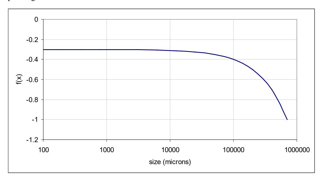
The equation which gave the best results is plotted in Figure 3 and is:
$$ f(x) = -(0.295 + x/1000000) $$ (12)
where x is the 80% passing size
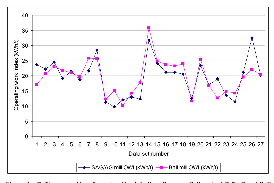
Using this equation, the mean value of Mi (as determined using plant data only) for the AG/SAG mill circuits was identical to that of the ball mill circuits. Individual results from the 27 data sets are plotted in Figure 4 and should be compared to the Bond operating work indices in Figure 2. It is clear that the new relationship significantly reduces the differences in operating work index between AG/SAG and ball mill circuits.
3.3 Determination of Mi Values
In a greenfield design situation equation 11 is of little or no value unless the \( M_i \) values can be determined from drill core samples as this is the only material which is normally available. Therefore a way of determining the Mi values from such drill core samples needs to be readily available.
Due to the different ways that rocks are broken in different comminution machines different \( M_i \) parameters are used for tumbling mills, crushers and HPGRs to reflect this (Morrell, 2009). Their associated \( M_i \) names are:
Tumbling mills (AG,SAG rod and ball mills) - \( M_{ia} \) , \( M_{ib} \)
Conventional crushers (jaw, gyratory and cone) - Mic
\( High \ Pressure \ Grinding \ Rolls \qquad \qquad - \qquad M_{ih} \)
Tumbling mills have two \( M_i \) parameters due to the very large range of particle sizes that are broken in these devices (ie typically in the range -150 mm + 45 microns) \( M_{ia} \) is related to "coarse" ore breakage and \( M_{ib} \) to "fine" ore properties. "Coarse" in this case is defined as spanning the size range from a P80 of 750 microns up to the P80 of the product of the last stage of crushing prior to grinding. In AG/SAG mills this may be as coarse as 150mm. "Fine" covers the size range from a P80 of 750 microns down to P80 sizes typically reached by conventional ball milling, ie about 45 microns.
\( M_{ia} \) , \( M_{ic} \) and \( M_{ih} \) values are provided as a standard output from a SMC Test®, which is a laboratory test designed to accommodate small diameter drill core samples. A general description of the test is given in Appendix 1. Most metallurgical laboratories around the world offer this test.
\( M_{ib} \) values are determined using the data generated by a conventional Bond ball mill work index test using the following equation (Morrell, 2006):
$$ M_{ib} = \frac{18.18}{P_1^{0.295} (Gbp) \left( p_{80}^{f(p_{80})} - f_{80}^{f(f_{80})} \right)} $$ (13)
where
\( M_{ib} \) = fine ore work index (kWh/tonne)
\( P_1 \) = closing screen size in microns
Gbp = net grams of screen undersize per mill revolution
\( p_{80} = 80\% \) passing size of the product in microns
\( f_{80} \) = 80% passing size of the feed in microns
f(x) = -(0.295 + x/1000000); where x is the 80% passing size
Note that the Bond ball work index test should be carried out with a closing screen size which gives a final product P80 similar to that intended for the full scale circuit.
4 PRACTICAL APPLICATION
4.1 General
Most comminution circuits comprise a number of different machines each handling the size reduction of a particular part of the size distribution spectrum in a stepwise manner. Hence considering the feed and the product of the overall comminution circuit the total specific energy \( (W_T) \) is given by the sum of each of these steps:
where
\( W_a \) = specific energy to grind coarser particles in tumbling mills
\( W_b \) = specific energy to grind finer particles in tumbling mills
\( W_c \) = specific energy for conventional crushing
\( W_h \) = specific energy for HPGRs
\( W_s \) = specific energy correction for size distribution
Clearly only the W values associated with the relevant equipment in the circuit being studied are included in equation 14.
4.2 Tumbling Mills
For coarse particle grinding in tumbling mills equation 11 is written as:
where
\( K_1 = 1.0 \) for all circuits that do not contain a recycle pebble crusher and 0.95 where circuits do have a pebble crusher
\( x_1 \) = \( P_{80} \) in microns of the product of the last stage of crushing before grinding
\( x_2 = 750 \text{ microns} \)
\( M_{ia} \) = Coarse ore work index and is provided directly by SMC Test®
For fine particle grinding equation 11 is written as:
where
\( x_2 = 750 \text{ microns} \)
\( x_3 = P_{80} \) of final grind in microns
\( M_{ib} \) = fine ore work index obtained from Bond ball work index test data
4.3 Conventional Crushers
Equation 11 for conventional crushers is written as:
where
\( K_2 = 1.0 \) for all crushers operating in closed circuit with a classifying screen. If the crusher is in open circuit, eg pebble crusher in a AG/SAG circuit, \( K_2 \) takes the value of 1.19.
\( x_1 = P_{80} \) in microns of the circuit feed
\( x_2 = P_{80} \) in microns of the circuit product
\( M_{ic} \) = Crushing ore work index and is provided directly by SMC Test®
4.4 HPGR
Equation 11 for HPGRs is written as:
where
\( K_3 = 1.0 \) for all HPGRs operating in closed circuit with a classifying screen. If the HPGR is in open circuit, \( K_3 \) takes the value of 1.19.
\( x_1 = P_{80} \) in microns of the circuit feed
\( x_2 \) = \( P_{80} \) in microns of the circuit product
\( M_{ih} \) = HPGR ore work index and is provided directly by SMC Test®
4.5 Tumbling Mill Specific Energy Correction for Size Distribution (Ws)
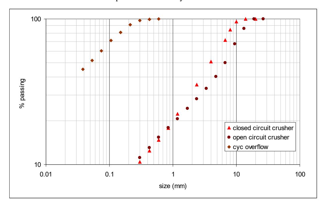
Implicit in the approach described in this paper is that the feed and product size distributions are parallel and linear in log-log space. Where they are not, corrections need to be made. By and large, such corrections are most likely to be necessary (or are large enough to be warranted) when evaluating circuits in which closed circuit secondary/tertiary crushing is followed by ball milling. This is because such crushing circuits tend to produce a product size distribution which is relatively steep when compared to the ball mill circuit cyclone overflow. This is illustrated in Figure 5, which shows measured distributions from an open and closed crusher circuit as well as a ball mill cyclone overflow. The closed circuit crusher distribution can be seen to be relatively steep compared with the open circuit crusher distribution and ball mill cyclone overflow. Also the open circuit distribution more closely
follows the gradient of the cyclone overflow. If a ball mill circuit were to be fed 2 distributions, each with same P80 but with the open and closed circuit gradients in Figure 5, the closed circuit distribution would require more energy to grind to the final P80. How much more energy is required is difficult to determine. However, for the purposes of this approach it has been assumed that the additional specific energy for ball milling is the same as the difference in specific energy between open and closed crushing to reach the nominated ball mill feed size. This assumes that a crusher would provide this energy. However, in this situation the ball mill has to supply this energy and it has a different (higher) work index than the crusher (ie the ball mill is less energy efficient than a crusher and has to input more energy to do the same amount of size reduction). Hence from equation 18, to crush to the ball mill circuit feed size \( (x_2) \) in open circuit requires specific energy equivalent to:
$$ W_c = 1.19 * M_{ic} 4 \left( x_2^{f(x_2)} - x_1^{f(x_1)} \right) $$ (20)
For closed circuit crushing the specific energy is:
$$ W_c = 1 * M_{ic} 4 \left( x_2^{f(x_2)} - x_1^{f(x_1)} \right) $$ (21)
The difference between the two (eq 20 - eq 21) has to be provided by the milling circuit with an allowance for the fact that the ball mill has to do the size reduction work and not the crusher. This is what is referred to in equation 14 as \( W_s \) and from equations 20 and 21 is represented by:
$$ W_s = 0.19 * M_{ia} 4 \left( x_2^{f(x_2)} - x_1^{f(x_1)} \right) $$ (22)
Note that in equation 22, \( M_{\rm ic} \) is replaced with \( M_{\rm ia} \) - the coarse particle tumbling mill grinding work index – to take account of the fact that the ball mill is doing the grinding work and not the crusher.
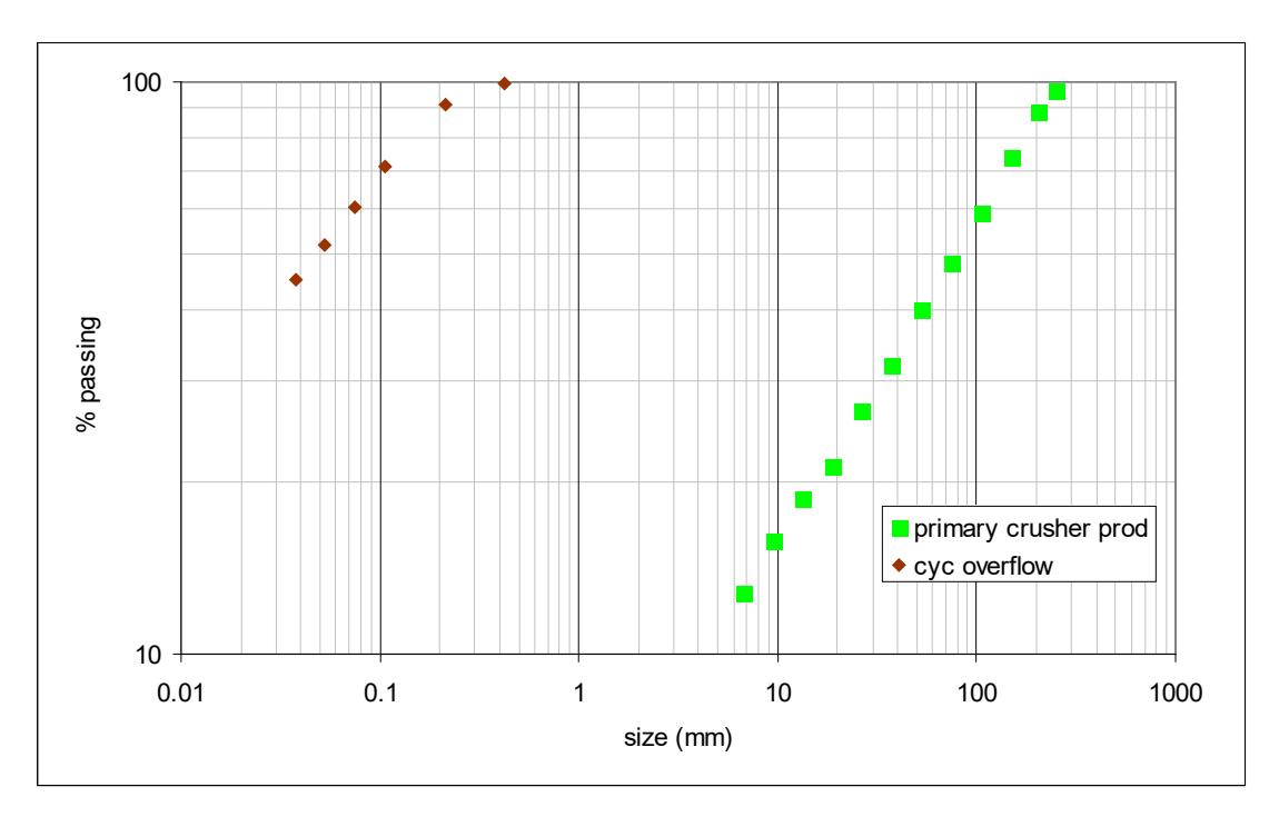
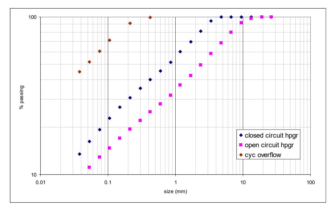
In AG/SAG-based circuits the need for Ws appears to be unnecessary as Figure 6 illustrates. Primary crusher feeds often have the shape shown in Figure 6 and this has a very similar gradient to typical ball mill cyclone overflows. A similar situation appears to apply with HPGR product size distributions, as illustrated in Figure 7. Interestingly the author's data show that for HPGRs, closed circuit operation appears to require a lower specific energy to reach the same P80 as in open circuit, even though the distributions for open and closed circuit look to have almost identical gradients. Closer examination of the distributions in fact shows that in closed circuit the final product tends to have progressively less material in the sub-100 micron range, which may account for the different energy requirements between the two modes of operation. It is also possible that recycled material in closed circuit is inherently weaker than new feed, as it has already passed through the HPGR previously and may have sustained micro-cracking. A reduction in the Bond ball mill work index as measured by testing HPGR products compared to the Bond ball mill work index of HPGR feed has been noticed in many cases in the laboratory (Stephenson,1997; Daniel,2007; Shi et al.,2006) and hence there is no reason to expect the same phenomenon would not affect the recycled HPGR screen oversize.
It follows from the above arguments that in HPGR circuits, which are typically fed with material from closed circuit secondary crushers, a similar feed size distribution correction should also be applied. However, as the secondary crushing circuit uses a relatively small amount of energy compared to the rest of the circuit (as it crushes to a relatively coarse size) the magnitude of the size distribution correction is relatively small – much smaller than the error associated with the technique - and hence may be omitted in calculations.
4.6 Enhancements for Crushing/HPGR Treatment of Coarse Feeds
New crushing and HPGR data have been recently acquired which have provided the opportunity to enhance the range of applications originally considered by equation 11, notably size reduction of relatively coarse feeds (Morrell, 2010). This is achieved through the addition of a size-dependent ore hardness term (S) which takes account of the reduction in rock strength that becomes significant in crushers handling run-of-mine feeds, though is also apparent in secondary crushing applications as well. Analysis of these new data indicates that this coarse particle ore hardness parameter (S) can be described by the general form shown in equation 1, and not only improves the accuracy of specific energy predictions of relevant crushing circuits but also those of full scale HPGR circuits. For conventional crushing the parameter should only be used in primary and secondary crushing circuits. In the case of tertiary and AG/SAG mill pebble crusher circuits its use should normally not be necessary. For HPGRs the parameter should improve accuracy in cases where the circuit feed P80 is in excess of 20-25mm.
Where
S = coarse ore hardness parameter
\( K_s \) = machine-specific constant that takes the value of 55 for conventional crushers and 35 in the case of HPGRs
\( x_1 = P_{80} \) in microns of the circuit feed
\( x_2 \) = \( P_{80} \) in microns of the circuit product
The specific energy equation for conventional crushers now becomes:
$$ W_c = S_c K_2 M_{ic} 4 \left( x_2^{f(x_2)} - x_1^{f(x_1)} \right) $$ (24)
Where
Wc = specific energy of the circuit (kWh/tonne)
\( S_c = 55.(x_1.x_2)^{-0.2} \) for primary and secondary crushing; otherwise it is set to unity
\( K_2 \) = 1.0 for all crushers operating in closed circuit with a classifying screen. If the crusher is in open circuit, eg pebble crusher in a AG/SAG circuit, \( K_2 \) takes the value of 1.19.
\( M_{ic} \) = Crushing ore work index and is provided directly by SMC Test®
For HPGRs the specific energy equation now is:
Where
\( W_h \) = specific energy of the circuit (kWh/tonne)
\( S_h = 35.(x_1.x_2)^{-0.2} \) where the HPGR feed P80 is greater than 20-25mm; otherwise it is set to unity
K3 = 1.0 for all HPGRs operating in closed circuit with a classifying screen. If the HPGR is in open circuit, K3 takes the value of 1.19.
Mih = HPGR ore work index and is provided directly by SMC Test®
4.7 Reduction in Bond Ball Work Index due to HPGR Treatment
As mentioned in the previous section, laboratory experiments have been reported by various researchers in which the Bond ball work index of HPGR products is less than that of the feed. The amount of this reduction appears to vary with both material type and the pressing force used and has been attributed to the influence of micro-cracking. Observed reductions in the Bond ball work index have typically been in the range 0-10%. The equations used in this paper makes no specific allowance for the influence of micro-cracking. However, if HPGR products are available which can be used to conduct Bond ball work index tests on, then Mib values obtained from such tests can be used in equation 16. If micro-cracking of the HPGR products has taken place then the resultant Mib value will reflect its effect. Alternatively the Mib values from Bond ball mill work index tests on HPGR feed material can be reduced by an amount that the reader thinks is appropriate. Currently, published data on full scale HPGR/ball mill circuits is very sparse and hence it is not yet possible to determine the extent to which laboratory test results on reductions in the Bond ball work index are translated into reductions in the ball mill circuit operating work index at the full scale. For this reason the author suggests that at least until more full scale data can be collected and analysed reductions in the Mib value due to micro-cracking are limited to 5%.
5 VALIDATION
5.1 General
The equations described in the previous sections were applied to a range of comminution circuits in the following way. Relevant data from these circuits were collected during surveys (audits) and included feedrates, power draws, as well as feed and product size distributions. Samples of fresh feed were also taken. This material was then sent to an appropriate metallurgical laboratory, where the relevant size fractions were extracted for SMC and Bond ball work index testing. On the basis of the measured feed and product size distributions, as well as the Mia and Mib ,Mic and Mih values obtained from laboratory testing of the feed samples, the overall specific energies of the circuits were predicted and compared with the measured values.
5.2 Tumbling Mills
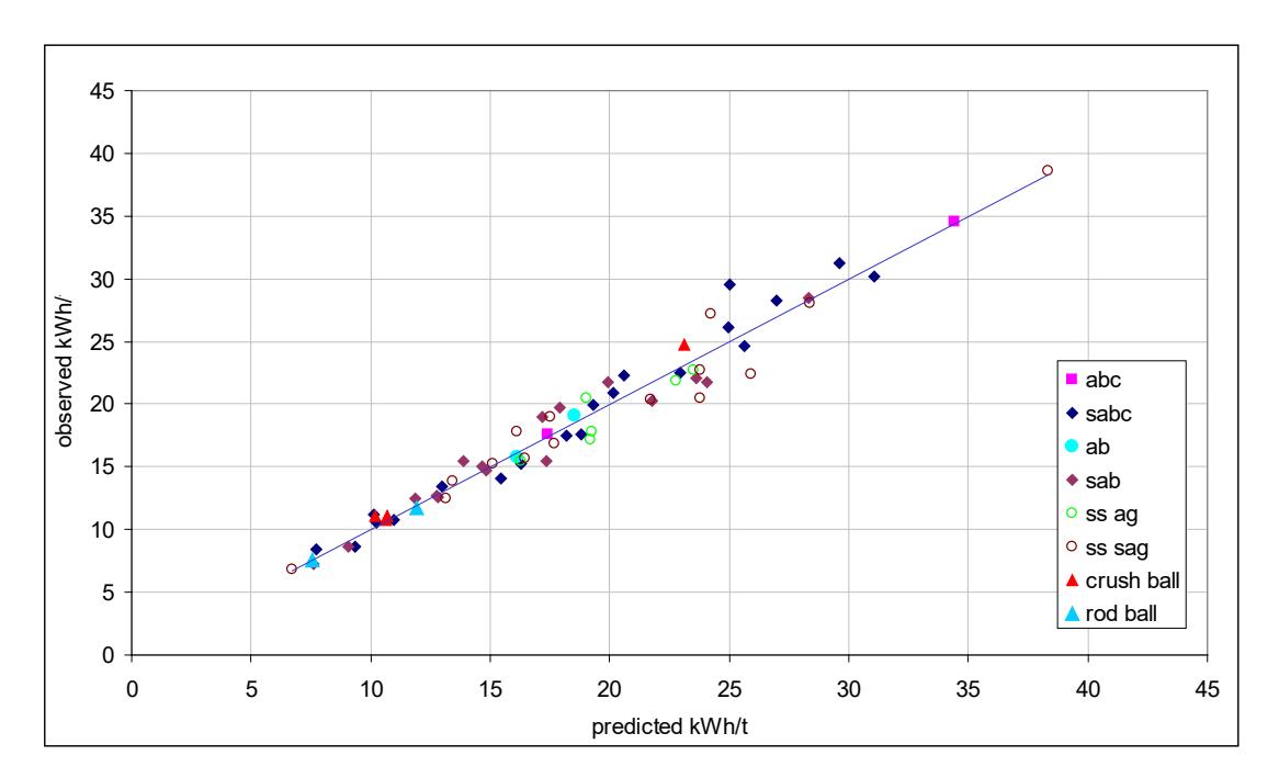
Data were collected from 65 tumbling mill circuits. The predicted specific energies compared with the measured values are shown in Figure 8. In all cases the specific energy relates to the tumbling mills contributing to size reduction from the product of the final stage of crushing/HPGR to the cyclone overflow. Data are presented in terms of equivalent specific energy at the pinion. In determining what these values were on each of the plants in the data base it was assumed that power at the pinion was 93.5% of the measured gross (motor input) power, this figure being typical of what is normally accepted as being reasonable to represent losses across the motor and gearbox. For gearless drives (so-called wrap-around motors) a figure of 97% was used.
5.3 Conventional Crushers
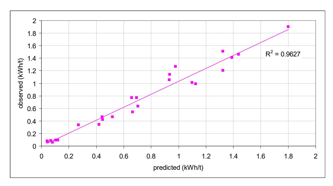
Validation of equation 24 used data from 4 primary, 6 secondary, 6 tertiary and 9 AG/SAG mill pebble crushing circuits. Observed vs predicted specific energies are given in Figure 9. The observed specific energies were calculated from the crusher throughput and the net power draw of the crusher as defined by:
$$ Net Power = Motor Input Power - No Load Power $$ (26)
No-load power tends to be relatively high in conventional crushers and hence net power is significantly lower than the motor input power. From examination of the 18 crusher data sets the motor input power was found to be on average 25% higher than the net power.
5.4 HPGRs
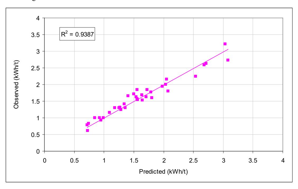
Validation of equation 25 for HPGRs used data from 19 different circuits (36 data sets) including laboratory, pilot and industrial scale equipment. Observed vs predicted specific energies are given in Figure 10. The data relate to HPGRs operating with specific grinding forces typically in the range 2.5-3.5 N/mm2 . The observed specific energies relate to power delivered by the roll drive shafts. Motor input power for full scale machines is expected to be 8-10% higher.
6 SUMMARY OF EQUATIONS AND WORKED EXAMPLES
6.1 Summary of Equations
The relevant equations to predict the comminution circuit specific energy are summarised in the following section
where
W = Specific energy (kWh/tonne)
K = Constant chosen to balance the units of the equation
\( M_i \) = Index related to how an ore breaks in the comminution device (kWh/t)
\( x_2 = 80\% \) passing size for the product
\( x_1 = 80\% \) passing size for the feed
\( f(x_i) = -(0.295 + x_i/1000000) \)
where
\( W_T \) = Total specific energy
\( W_a \) = specific energy to grind coarser particles in tumbling mills
\( W_b \) = specific energy to grind finer particles in tumbling mills
\( W_c \) = specific energy for conventional crushing
\( W_h \) = specific energy for HPGRs
\( W_s \) = specific energy correction for size distribution
$$ W_a = K_1 M_{ia} 4 \left( x_2^{f(x_2)} - x_1^{f(x_1)} \right) $$ (iii)
where
\( K_1 = 1.0 \) for all circuits that do not contain a recycle pebble crusher and 0.95 where circuits do have a pebble crusher
\( x_1 = P_{80} \) in microns of the product of the last stage of crushing before grinding
\( x_2 = 750 \text{ microns} \)
\( M_{ia} \) = Coarse ore work index and is provided directly by SMC Test®
$$ W_b = M_{ib} 4 \left( x_3^{f(x_3)} - x_2^{f(x_2)} \right) $$ (iv)
where
\( x_2 = 750 \text{ microns} \)
\( x_3 = P_{80} \) of final grind in microns
\( M_{ib} \) = Provided by data from the standard Bond ball work index test using the following equation
$$ M_{ib} = \frac{18.18}{P_1^{0.295} (Gbp) \left( p_{80}^{f(p_{80})} - f_{80}^{f(f_{80})} \right)} $$ (v)
where
\( M_{ib} \) = fine ore work index (kWh/tonne)
\( P_1 \) = closing screen size in microns
Gbp = net grams of screen undersize per mill revolution
\( p_{80} = 80\% \) passing size of the product in microns
\( f_{80} \) = 80% passing size of the feed in microns
$$ W_c = S_c K_2 M_{ic} 4 \left( x_2^{f(x_2)} - x_1^{f(x_1)} \right) $$ (vi)
where
\( S_c \) = 55. \( (x_1.x_2)^{-0.2} \) for primary and secondary crushing; in all other cases \( S_c = 1 \)
\( K_2 = 1.0 \) for all crushers operating in closed circuit with a classifying screen. If the crusher is in open circuit, eg pebble crusher in a AG/SAG circuit, \( K_2 \) takes the value of 1.19.
\( x_1 = P_{80} \) in microns of the circuit feed
\( x_2 \) = \( P_{80} \) in microns of the circuit product
\( M_{ic} \) = Crushing ore work index and is provided directly by SMC Test®
$$ W_h = S_h K_3 M_{ih} 4 \left( x_2^{f(x_2)} - x_1^{f(x_1)} \right) $$ (vii)
where
\( S_h = 35.(x_1.x_2)^{-0.2} \) in cases where \( x_1 > 25 \) mm; in all other cases \( S_h = 1 \)
\( K_3 = 1.0 \) for all HPGRs operating in closed circuit with a classifying screen. If the HPGR is in open circuit, \( K_3 \) takes the value of 1.19.
\( x_1 = P_{80} \) in microns of the circuit feed
\( x_2 \) = \( P_{80} \) in microns of the circuit product
\( M_{ih} \) = HPGR ore work index and is provided directly by SMC Test®
$$ W_s = S_c * 0.19 * M_{ia} 4 \left( x_2^{f(x_2)} - x_1^{f(x_1)} \right) $$ (viii)
where
x1 = P80 in microns of the circuit feed
x2 = P80 in microns of the circuit product
Mia = Coarse ore work index and is provided directly by SMC Test®
6.2 Worked Examples
The following worked examples are presented to assist the reader in understanding how the energy equations are used in practical situations. Reference is made throughout to the relevant equations as numbered i-viii in section 6.1.
A SMC Test® and Bond ball work index test were carried out on an ore sample. The following results were obtained:
SMC Test®:
Mia = 19.4 kWh/t
Mic = 7.2 kWh/t
Mih = 13.9 kWh/t
Bond test (carried out with a 150 micron closing screen):
Mib = 18.8 kWh/t
Three circuits are to be evaluated:
- SABC
- HPGR/ball mill
- Conventional crushing/ball mill
The overall specific energy to reduce a ROM F80 of 450mm to a final product P80 of 106 microns is required to be estimated. Assume the first stage in all circuits will be an open circuit primary crusher set to give a P80 of 100mm.
6.2.1 SABC Circuit
Primary crusher
Combining eq i and vi:
$$ W_c = 55 * (100000 * 450000)^{-0.2} * 1.19 * 7.2 * 4 * (100000^{-(0.295 + 100000/1000000)} - 450000^{-(0.295 + 450000/1000000)}) $$ $$ = 0.15 \text{ kWh/t} $$
Coarse particle tumbling mill specific energy
Combining eq i and iii:
$$ W_a = 0.95*19.4*4*\left(750^{-(0.295+750/1000000)} - 100000^{-(0.295+100000/1000000)}\right) $$ $$ = 9.63 \text{ kWh/t} $$
Fine particle tumbling mill specific energy
Combining eq i and iv:
$$ W_b = 18.8 * 4 * \left(106^{-(0.295 + 106/1000000)} - 750^{-(0.295 + 750/1000000)}\right) $$ = 8.36 kWh/t
Pebble crusher specific energy
In this circuit it is assumed that the pebble crusher feed P80 is 52.5mm. As a rule of thumb this value can be estimated by assuming that it is 0.75 of the nominal pebble port aperture (in this case the pebble port aperture is 70mm). The pebble crusher is set to give a product P80 of 12mm. The pebble crusher feed rate is expected to be 25% of new feed tph.
Combining eq i and vi:
- = 1.07 kWh/t when expressed in terms of the crusher feed rate
- = 1.07 * 0.25 kWh/t when expressed in terms of the SABC circuit new feed
rate
= 0.27 kWh/t of SAG mill circuit new feed
Total net comminution specific energy:
From eq ii:
$$ W_T = 0.15+9.63 + 8.36 + 0.27 $$
kWh/t
= 18.41 kWh/t
6.2.2 HPGR/Ball Milling Circuit
In this circuit primary crusher product is reduced to a HPGR circuit feed P80 of 35 mm by closed circuit secondary crushing. The HPGR is also in closed circuit and reduces the 35 mm feed to a circuit product P80 of 4 mm. This is then fed to a closed circuit ball mill which takes the grind down to a P80 of 106 microns.
Primary crusher
Combining eq i and vi:
$$ W_c = 55 * (100000 * 450000)^{-0.2} * 1.19 * 7.2 * 4 * (100000^{-(0.295 + 100000/1000000)} - 450000^{-(0.295 + 450000/1000000)}) $$ $$ = 0.15 \text{ kWh/t} $$
Secondary crushing specific energy
Combining eq i and vi:
$$ W_c = 55 * (35000 * 100000)^{-0.2} * 1 * 7.2 * 4 * (35000^{-(0.295 + 35000/1000000)} - 100000^{-(0.295 + 100000/1000000)}) $$ $$ = 0.41 \text{ kWh/t} $$
HPGR specific energy
Combining eq i and vii:
= 2.38 kWh/t
Coarse particle tumbling mill specific energy
Combining eq i and iii:
$$ W_a = 1*19.4*4* \left(750^{-(0.295+750/1000000)} - 4000^{-(0.295+4000/1000000)}\right) $$ = 4.45 kWh/t
Fine particle tumbling mill specific energy
Combining eq i and iv:
$$ W_b = 18.8 * 4 * \left(106^{-(0.295+106/1000000)} - 750^{-(0.295+750/1000000)}\right) $$ = 8.36 kWh/t
Total net comminution specific energy:
From eq ii:
$$ W_T = 0.15+0.41+2.38+4.45+8.36 $$
kWh/t
= 15.75 kWh/t
6.2.3 Conventional Crushing/Ball Milling Circuit
In this circuit primary crusher product is reduced in size to a P80 of 6.5 mm via a secondary/tertiary crushing circuit (closed). This is then fed to a closed circuit ball mill which grinds to a P80 of 106 microns.
Primary crusher
Combining eq i and vi:
$$ W_c = 55 * (100000 * 450000)^{-0.2} * 1.19 * 7.2 * 4 * (100000^{-(0.295 + 100000/1000000)} - 450000^{-(0.295 + 450000/1000000)}) $$ $$ = 0.15 \text{ kWh/t} $$
Secondary/tertiary crushing specific energy
Combining eq i and vi:
$$ W_c = 55 * (6500 * 100000)^{-0.2} * 1 * 7.2 * 4 * (6500^{-(0.295 + 6500/1000000)} - 100000^{-(0.295 + 100000/1000000)}) $$ $$ = 1.65 \text{ kWh/t} $$
Coarse particle tumbling mill specific energy
Combining eq i and iii:
$$ W_a = 1*19.4*4* \left(750^{-(0.295+750/1000000)} - 6500^{-(0.295+6500/1000000)}\right) $$ = 5.45 kWh/t
Fine particle tumbling mill specific energy
Combining eq i and iv:
$$ W_b = 18.8 * 4 * \left(106^{-(0.295+106/1000000)} - 750^{-(0.295+750/1000000)}\right) $$ = 8.36 kWh/t
Tumbling mill size distribution correction
From eq viii:
$$ W_S = 55 * (6500 * 100000)^{-0.2} * 0.19 * 19.4 * 4 * (6500^{-(0.295 + 6500/1000000)} - 100000^{-(0.295 + 100000/1000000)}) $$ $$ = 0.84 \text{ kWh/t} $$
Total net comminution specific energy:
From eq ii:
$$ W_T $$
= 0.15+1.65+5.45 + 8.36 + 0.84 kWh/t
= 16.45 kWh/t
7 REFERENCES
Barratt, D. J. and Allan, M.J., 1986, Testing for Autogenous and Semi-autogenous Grinding: a Designer's Point of View. Minerals and Metallurgical Processing. May, pp 65-74
Blaskett K.S., 1969, Estimation of the Power Consumption in Grinding Mills. Proceeding of the Ninth Commonwealth Min. Metall., 3, pp 631-649.
Bond, F. C.,1952. The third theory of comminution, Trans AIME, vol 193, pp 484-494
Bond, F.C., 1961 (revised 1962). Crushing and Grinding Calculations. Allis-Chalmers publication O7R9235B
Bond, F.C., 1961. Crushing and Grinding Calculations. Brit. Chem Eng. Part I, 6 (6), 378- 385, Part II, 6 (8), 543-548
Griffith, A. A., 1920. The Phenomena of Rupture and Flow in Solids. Philosophical Transactions of the Royal Society of London (Series A: Mathematical and Physical), Vol A221, pp 163-197.
Hukki, R.T., 1962. Proposal for a solomnic settlement between the theories of von Rittinger, Kick and Bond, Trans AIME , vol 223, pp403-408.
Kick, F.,1885. Das Gesetz der proportionalen Widerstande und seine anwendung felix, Leipzig.
Larsen, C., Cooper, M. and Trusiak, A., 2001. design and Operation of Brunswick's AG/SAG Circuit, Proc International Autogenous and Semi Autogenous Grinding Technology, Vancouver, vol IV pp 350-367.
Levin, J., 1989. Observation on the Bond Standard Grindability Test, and a Proposal for a Standard Grindability Test for Fine Materials. SAIMM, vol 89, n0.1, pp13-21.
Morrell, S., 2004. An Alternative Energy-Size Relationship To That Proposed By Bond For The Design and Optimisation Of Grinding Circuits. International Journal of Mineral Processing, 74, 133-141.
Morrell, S., 2006. Rock Characterisation for High Pressure Grinding Rolls Circuit Design, Proc International Autogenous and Semi Autogenous Grinding Technology,Vancouver, vol IV pp 267-278.
Morrell,S., 2008, A method for predicting the specific energy requirement of comminution circuits and assessing their energy utilisation efficiency, Minerals Engineering, Vol. 21 , No. 3.
- S. Morrell, 2010 .Predicting the specific energy required for size reduction of relatively coarse feeds in conventional crushers and high pressure grinding rolls, Minerals Engineering, Vol. 23 , No. 2.
- S. Morrell, 2009. Predicting the overall specific energy requirement of crushing, high pressure grinding roll and tumbling mill circuits, Minerals Engineering, Vol. 22 , No. 6, 2009 Morrell, S., Johnson, G. and Revy, T., 1991. A comparison through observation and simulation of the power utilisation and performance of two dissimilar comminution plants. Fourth Mill Operators' Conference, Aus.IMM Burnie, pp157-160. March.
Morrell, S., Valery, W., Banini, G. and Latchireddi, S., 2001. Developments in AG/SAG Mill Modelling Proc International Autogenous and Semi Autogenous Grinding Technology, Vancouver, vol IV pp 71-84.
von Rittinger, P. R., 1867. Lehrbuch der Aufbereitungskunde, Ernst and Korn, Berlin,
Rowland, C.A.Jnr and Kjos, D.M., 1978 (revised 1980). Rod and Ball Mills. Mineral Processing Plant Design. Mular and Bhappu (editors), SME, Chapter 12, pp 239-278.
Rumph, H., 1973. Physical Aspects of Comminution and New Formulation of a Law of Comminution, Powder Technology, 7, pp 145-159.
Tavares, L. M. and King, R. P., 1998. Single-particle Fracture under Impact Loading. International Journal of Mineral Processing, Vol. 54, pp 1-28.
Walker, W. H., Lewis W K, McAdams W H, and Gilliland E K., 1937. Principles of Chemical Engineering, New York.
Weibull, W., 1939. A statistical theory of strength of materials. Proceedings of the royal Swedish Academy of Engineering Science (Ingeniorsvetenskapsakademiens Handlingar), No 151
Daniel, M.J., 2007, Energy efficient mineral liberation using HPGR technology, PhD Thesis, Julius Kruttschnitt Mineral Research Centre, Department of Mining and Metallurgical Engineering, University of Queensland
Stephenson, I.;1997, The downstream effects of high pressure grinding rolls processing, PhD Thesis, Julius Kruttschnitt Mineral Research Centre, Department of Mining and Metallurgical Engineering, University of Queensland.
Schonert, K., 1991. Advances in comminution fundamental, and impacts on technology. XVII International Mineral Processing Congress, Dresden, Volume 1,: pp 1-21.
Shi, F., Lambert, S., Daniel, M.J., 2006, Measurement of the effect of HPGR treating platinum ores. SAG 2006, Vancouver, 23-27 September 2006.
APPENDIX 1 – About the SMC Test®
The SMC Test® was developed to make use of relatively small samples, both in terms of quantity and particle size and to be versatile so as to make as much use as possible of whatever samples are available for testing. As a result it is able to accommodate a wide range of particle sizes either in core or crushed form. The test is applied to particles of a particular size, the size chosen depending on the type and quantity of sample available. The choices of particle size that can be used in the SMC Test are shown in Table 1. Sample sources can be from a range of core sizes as given in Table 2. Typically either the 31.5+26.5mm or – 22.4+19mm particle sizes are chosen as these are easily extractable from HQ and NQ cores respectively, and these tend to be the most popular core sizes used. When sample availability is very limited, quartered (slivered) core samples are cut using a diamond saw (Figure A1). This results in sample mass requirements as low as 2-2.5 kgs in total. However, where core is available in sufficient quantity (10-15 kgs) it can be crushed and the appropriate size fraction extracted eg quartered PQ core or half HQ or whole NQ could be crushed to extract (say) – 22.4+19mm specimens suitable for testing etc (Figure A2).
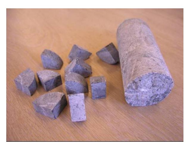
Figure A1 – Pieces Cut from a Drill Core Using a Diamond Saw
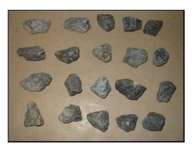
Figure A2 – Pieces Obtained by Crushing Drill Core
| Particle size |
| (mm) |
| -45+37.5 |
| -31.5+26.5 |
| -22.4-19 |
| -16+13.2 |
Table A1 – Particle Size Ranges Typically used in an SMC Test
| Nominal | |||||||
|---|---|---|---|---|---|---|---|
| Core | diam. | ||||||
| mm | |||||||
| PQ | 85 | ||||||
| HQ | 63.5 | ||||||
| NQ | 47.6 |
|---|---|
| BQ | 36.5 |
| AQ | 27 |
Table A2 – Core Sizes Suitable for Use in an SMC Test
Once the core has been cut or crushed into the chosen particle size range, 100 specimens are selected. The mean specific gravity of the specimens is then determined then they are divided into five equal lots of 20 pieces. Each lot is then broken in an impact device using a range of closely controlled energies. A suitable impact device is the JKMRC's drop-weight tester (Napier-Munn et al, 1996). After breakage the products are collected and sized on a sieve whose aperture is related to the original particle size. The % of undersize from sieving the broken products is plotted against the input energy.
These results are then used to determine the so-called drop-weight index (DWi) which is a measure of the strength of the rock. It is directly related to the JK rock breakage parameters A, b and ta as well as the JK crusher model's t10-Ecs matrix, all of which are generated as part of the standard report output from the test. These values can then be used to simulate crushing and grinding circuits using JKTech's simulator – JKSimMet. Correlations also exist between the DWi and point load index (IS50) making it valuable in Mine-to-mill studies as well.
The SMC Test® also provides the comminution indices Mia, Mih and Mic ,which are routinely reported when a test is carried out (see Table A3 below).
|
Power-based Indices
AG/SAG Model Parameters |
Crusher Model Matrix | ||||||||||||||||
|---|---|---|---|---|---|---|---|---|---|---|---|---|---|---|---|---|---|
| particle size (mm) | |||||||||||||||||
| 14.5 | 14.5 | 14.5 | 28.9 | 28.9 | 28.9 | 57.8 | 57.8 | 57.8 | |||||||||
| t10 | |||||||||||||||||
| ID | DWi | Mia | Mih | Mic | A | b | sg | ta | 10 | 20 | 30 | 10 | 20 | 30 | 10 | 20 | 30 |
| kWh/m3 | kWh/t kWh/t | kWh/t | kWh/t kWh/t kWh/t kWh/t kWh/t kWh/t kWh/t kWh/t kWh/t | ||||||||||||||
| A | 12.16 | 25.2 | 21.0 | 10.9 | 87.9 | 0.31 | 3.36 | 0.21 | 0.51 | 1.11 | 1.83 | 0.39 | 0.82 | 1.31 | 0.29 | 0.61 | 0.95 |
| B | 13.33 | 26.5 | 22.5 | 11.6 | 84.3 | 0.31 | 3.44 | 0.19 | 0.55 | 1.19 | 1.96 | 0.41 | 0.88 | 1.40 | 0.31 | 0.65 | 1.02 |
| C | 5.54 | 17.6 | 12.5 | 6.5 | 50.0 | 0.93 | 2.57 | 0.47 | 0.31 | 0.66 | 1.09 | 0.23 | 0.49 | 0.78 | 0.17 | 0.36 | 0.57 |
Table A3 – Example of Standard Output Report from SMC Test®