



The content on this page was automatically generated from the PDF publication document and may contain errors or inaccuracies. Please refer to the original PDF for the most accurate information.
Power Draw of Grinding Mills — Its Measurement and Prediction
S Morrell1
ABSTRACT
In recent years the Julius Kruttschnitt Mineral Research Centre (JKMRC) has developed mathematical models for accurately predicting the power draw of ball, semi-autogenous (SAG) and fully autogenous (AG) mills. In the course of this work data on over 70 such mills in Australia were collected and analysed. These data covered a very wide range of design and operating conditions and can be considered a good cross-section of mills operating in the minerals processing industry in this country.
This paper presents an overview of these data, highlighting the variations in design and operating conditions. The importance to operators of having accurate measurements of power draw as well as mill dimensions, charge levels, etc is also discussed. Problems associated with obtaining accurate measurements are described as well as methods and procedures which can be followed to ensure errors are kept to a minimum. Using the JKMRC's power model the effects of design and operating conditions are illustrated, with particular reference to the influence of measurement errors.
INTRODUCTION
The energy consumed by milling in the minerals processing industry accounts for a major part of the operating cost of a plant (Morrell et al, 1991). For design and optimisation purposes it is therefore of great importance that power draw of mills can be accurately predicted. To this end the Julius Kruttschnitt Mineral Research Centre (JKMRC) has recently completed a research program which has resulted in the development of a mathematical model for predicting the power draw of ball, autogenous (AG) and semi-autogenous (SAG) mills. However, without good quality comprehensive data with which to validate a model, it is of little or no practical value. Therefore to ensure that the model had a proven ability to accurately predict the power draw of industrial mills, an extensive database was assembled.
This paper presents an overview of the the JKMRC power model and describes the database that was generated to validate it. In addition the problems that were encountered with collecting good quality power draw and associated data are described.
OVERVIEW OF JKMRC POWER MODEL
The rotation of a cylindrical tumbling mill moves the charge it contains and in so doing consumes energy. determining the rate at which this energy is consumed (power) is in being able to describe the motion of the charge. Taggart's comments (1945) in this regard, which are still applicable today, are particularly relevant: 'Net power is not capable of analytic determination because of present ignorance of the internal dynamics of the tumbling load'. To address this deficiency, research recently completed at the JKMRC has resulted in the development of a number of mathematical models of the power draw of grinding mills (Morrell, 1993), based on consideration of the charge dynamics. The models vary in complexity, though each was designed to predict the power draw of industrial ball, SAG and AG mills. In this paper an overview of the version installed in the JKMRC's mineral process simulator — JKSimMet — is described. The complete equations of this model (C-model) can be found elsewhere (Morrell, 1993).
The model has the general form:
Gross power = No-load power + (k*Theoretical net power)
where:
k = calibration constant
The no-load power is determined from an empirical equation based on data from 14 mills. The net power equation is derived from a theoretical treatment and considers the charge shape and motion and the way they change with mill filling and speed. Of importance in the model, therefore, are the assumptions made about the charge shape and the way the charge moves. These are discussed in the following section.
General shape of the charge
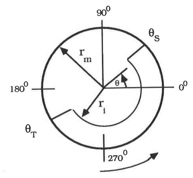
In a grate discharge mill the charge typically runs with the interstices in the grinding media (coarse) fraction rarely filled much beyond the point where all the voidage is occupied with slurry. The charge in such mills can be approximated as shown in Figure 1a. In the case of an overflow discharge mill slurry can only discharge once it overflows the discharge trunnion. Excess slurry is therefore present and gives rise to the second charge shape shown in Figure 1b. In this case a slurry pool exists in addition to the grinding media. The slurry pool is assumed to comprise a mixture of ore and water of the same density as the discharge slurry. The remainder of the charge is assumed to comprise the media whose interstices are fully occupied by slurry at the same density as the discharge slurry.
The presence of the slurry pool in the overflow mill results in a reduction of the power draw of the mill when compared to a grate discharge unit of the same size. In an empirical manner such differences in power draw have been incorporated in some mill power equations (Bond, 1962; Morrell, 1992). Mechanistically this effect can be considered to be caused by the assistance to Grate Discharge
Julius Kruttschnitt Mineral Research Centre (JKMRC), Isles Road, Indooroopilly Qld 4068.
Overflow Discharge
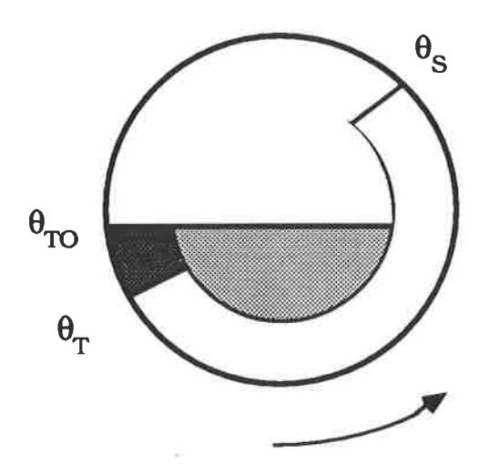
rotation that the slurry in the toe region provides. Only the toe region needs to be considered as far as the power draw is concerned. The symmetrical portion of the slurry pool lying vertically beneath the centre of rotation of the mill can be assumed not to exert a torque and hence does not contribute to the net power draw of the mill. However, it will provide an additional mass which, through increased frictional forces at the mill bearings, will cause an increase in mechanical losses. The magnitude of this effect, however, is considered to be small.
Power draw equations
The approach adopted in the C-model was to consider the rate at which potential and kinetic energy is generated within the charge. As power can be defined as energy per unit time, then the rate at which potential and kinetic energy is generated within the charge will provide an estimate of the mill power draw.
Thus with reference to Figure 1 it can be shown (Morrell. 1993) that the power associated with the cylindrical section (Pcylinder) is given by:
where:
L = length of cyclindrical section of the mill inside liners (m)
radial position (m)
radial position of charge inner surface (m)
radius of mill inside liners (m) \( r_m = \)
tangential velocity of a particle at radial distance angular displacement of shoulder position at the mill shell (rads.) angular displacement of toe position at the mill shell (rads.)
angular displacement of surface of slurry pool at the \( \theta_{TO} = \) toe (rads.)
density of total charge (t.m-3)
density of discharge pulp (t.m-3)
The variation in the shoulder and toe angles \( (\theta_S, \theta_T) \) as well as the velocity variation with radial position (Vr) are modelled empirically from observations of the charge in a glass laboratory mill. The slurry pool angle ( \( \theta_{TO} \) ) is assumed to be constant for overflow ball mills at 3.395 radians. In grate discharge mills it can usually be assumed that no slurry pool exists and hence \( \theta_{TO} = \theta_T \) . In some cases, however, typically where grate dicharge mills are run in closed circuit with a classifier, restrictions in grate flow capacity can cause a build-up of slurry in the mill which results in the formation of a slurry pool. This causes a reduction in power draw. Under such circumstances \( \theta_{TO} \) must be known before the power draw can be accurately predicted.
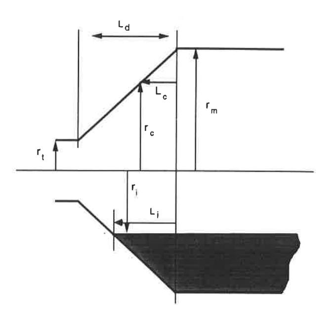
Some mills, particularly those with large diameter to length ratios, are not completely cylindrical, but have conical shaped ends. The charge in the cone-ends, as it tumbles, also draws power and must be added to that from the cylindrical section. However, account must be made of the fact that the filling varies with the longitudinal position in the cone. With reference to Figure 2, it can be shown (Morrell, 1993) that the power draw in the cone ends is given by:
where:
length of cone-end, measured from the cylindrical \( L_{c'} = \) section, at a radius of rc
length of charge surface within cone ends (m)
radial position (m)
radius of cone-end at a distance Lc from the cylindrical section (m) radial position of charge inner surface (m) tangential velocity of a particle at radial distance r (m.sec-1) angular displacement of shoulder position at the mill shell (rads) angular displacement of toe position at the mill shell (rads.) angular displacement of surface of slurry pool at the toe (rads) density of total charge (t.m-3) density of discharge pulp (t.m-3)
MILL POWER DRAW DATA
Although small laboratory mills provide an excellent test bed to determine the functional relationships between operating conditions and power draw, good quality full-scale plant data are required to determine whether such relationships hold at the industrial level.
Some industrial mill data can be found in the literature. However these are isolated cases and often lack sufficient detail to be useful for research purposes. The problem is compounded by the inherent difficulties in obtaining accurate data (Harris et al , 1985). To remedy this situation a mill database was assembled which could be confidently used to develop and validate the mill power models.
DATABASE STRUCTURE
The minimum details required in order to be able to predict a mill's power draw are:
- diameter (inside liners)
- cylinder length (inside liners)
- cone length (inside liners)
- speed
- discharge mechanism (grate or overflow)
- ball filling ) data are combined
- total filling (balls plus rock) } to give
- ore specific gravity. } the charge density
These details, together with the true power draw, were therefore sought for a wide a range as possible of mill dimensions, ore types and operating conditions. In the course of collecting these data from operational plants it became apparent that in a significant number of cases some of these data were either recorded incorrectly, not recorded at all and/or misunderstood by plant staff. Based on the experience from gathering these data the following comments are relevant concerning how and what data were collected.
Mill diameter
It is a fairly common misconception among plant personnel that the dimensions quoted in manufacturers manuals are inside liners. However, the dimensions usually quoted are inside shell and additionally a nominal new liner thickness may also be quoted. As the power draw is directly related to the inside liner dimension it is this measurement which needs to be taken. As the liners wear, however, the inside liner diameter will vary. Inside liner diameters can only be reliably obtained by direct measurement from inside the mill. In many cases these measurements were taken during the course of the data collection exercise. However in some instances inside shell diameters only were available. In such cases two nominal half-worn liner thicknesses were subtracted from the inside shell dimensions.
Mill length
Manufacturers will often quote an 'effective grinding length' (egl) for a mill. It is apparent that manufacturers differ in their definitions of what this is. In some cases it appears to be the length of the mill at the belly (ie the cylindrical section), inside the shell. In conical ended mills this is misleading as it effectively ignores the mill volume within the conical ends. Some manufacturers attempt to take account of this by specifying an egl which is in between the belly length and the centre-line lengths. In such cases it is difficult to establish how this length is determined.
The effect of having conical end-sections in a mill is to increase the volume of the grinding chamber, and hence the power draw, as compared to that of the cyclindrical section alone.
As the mill filling in the cylindrical section of the mill varies the length of the cone-ends which will be actively in use will also vary. Thus as the mill filling increases the active or effective length of the cone-ends will increase and hence so will the amount of power that the cone ends draw relative to the cylindrical section. It follows from this that the so called 'effective grinding length' is not invariant but is a function of the mill filling. The concept of the effective grinding length is therefore largely meaningless unless the filling to which it refers is also quoted. It is recommended that the practice of using the egl is avoided. While constructing the database engineering drawings were sought wherever possible and both belly and centre-line lengths determined. In some cases direct measurement was possible. As with the mill diameter, where actual measurements were not possible a nominal half worn liner thickness was assumed.
Mill speed
The most common method for reporting mill speed is the per cent of critical speed. This figure is often based on the rpm of the mill and a nominal inside liner dimension. As the per cent of critical speed is proportional to D0.5, the value calculated for the true inside liner dimension will therefore differ from this value. Wherever possible rpm data were recorded and the per cent of critical speed at the inside of the liners then calculated.
Ore specific gravity
In SAG and AG mills in particular, the ore SG has a significant effect on charge density and hence power draw. In all the data sets in the database the mean feed ore SG has been used. It is possible, however, that where blends of ore are being treated a harder constituent may be present of different SG to the remaining ore; in which case the SG of the ore in the mill will be different to that of the feed ore.
Mill filling
The mill filling is the volume of charge in the mill and hence has a significant effect on the power draw. In the case of ball mills the filling remains fairly steady over time, as it comprises mostly steel balls. It is common practice for operators to charge ball mills with steel balls according to a power set point. Due to the very stable power draws that are usually seen with ball mills, this procedure ensures that the mill is always charged to approximately the same level. In cases where direct measurements of the ball filling were not possible at the time when power readings were taken, plant historic records were used as a source for ball filling data. In AG/SAG mills, however, the feed ore contributes significant quantities of rock to the grinding media. As a result, changes in feed ore size distribution and hardness will affect the quantity of ore within the mill and hence the power draw. In all cases direct measurements of the loads were taken. In the case of AG/SAG mills this entailed running the mills under steady state then crash-stopping them under load. Access to the mill interior was then gained. Once inside the mill, measurements of the width of the charge in three places were taken together with inside-liner dimensions. From these measurements the load volume was calculated using simple geometry. In a number of cases access to the mill interior was denied. In such cases either photographs of the charge against the grate were taken and the charge level determined using engineering drawings of the grate and simple geometry. Alternatively a rod was inserted into the mill to measure the charge level below the feed trunnion.
SAG mill operations presented additional difficulties due to the ball filling which, being mixed with the ore charge, was difficult to estimate. In most cases mills were allowed to grind-out and the ball filling then measured. Due to the damage that this procedure can cause to the liners/lifters, however, this was not always possible. In such cases operator's estimates had to be used.
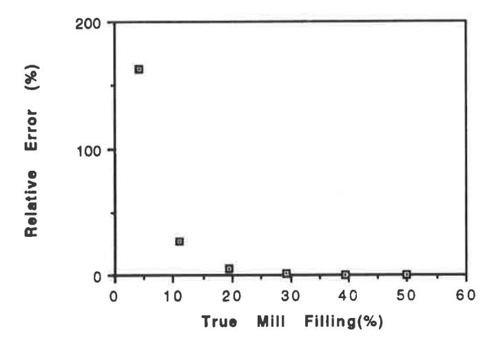
It was noticed that on most plants operational staff were found to favour the technique of measuring either the distance between the feed trunnion and the charge surface or the mill roof and charge surface. This technique can give rise to relatively high measurement errors. If measuring the charge width at a number of locations is a practical alternative this former technique should be avoided. It was also apparent that in some cases mill filling calculations had been made using the Allis Chalmer approximation rather than geometry. This approximation is as follows:
where
h = vertical distance between the charge surface and the mill roof, inside the liners.
D = mill diameter, inside the liners.
Although useful for relatively high mill fillings, this equation gives very large errors for smaller mill fillings. Figure 3 illustrates this in a plot of Equation 3 against the true mill filling.
Power draw
Plants vary widely in the type and complexity of their instrumentation. As a result power draw data were available from a range of devices including kWh meters, power transducers and ammeters. Where more than one source of power data was available at a particular site it was ensured that all sources gave similar readings. Where they did not, plant electrical staff were requested to investigate and correct the differences. Where this could not be done, the data were not included in the database. Where only one source of power measurement was available efforts were made to ensure that independent checks of the power reading accuracy had been made either prior to the field study or shortly afterwards.
It was alarming that in a significant number of cases the power draw indicated by control room instruments was significantly different to that subsequently found to be the case. If this problem is coupled to the additional one that some plants are unaware of their mill motor's true operational ceiling, a significant incidence of under-utilisation of mill capacity is indicated. It is strongly recommended that as a matter of routine the power measurement and indicator instruments on plants are checked for accuracy and operators are aware of the maximum power draw capability of their mill motors.
DATABASE DETAILS
In total 76 data sets were accumulated to test the validity of the model. Details of the range of tumbling mills covered in the database are given in Table 1.
| Ball Mills | SAG Mills | AG Mills | |
|---|---|---|---|
| Diameter (m) | 0.85-5.34 | 1.80-9.59 | 1.8–9.50 |
| Belly length inside liners (m) | 1.52-8.84 | 0.59–7.95 | 0.59–5.18 |
| Length/diameter ratio | 1.00-1.83 | 0.33-1.50 | 0.33-1.0 |
| Per cent of critical speed (%) | 60–83 | 48–89 | 72–75 |
| Ball filling (vol %) | 20-48 | 3–25 | 0 |
| Total filling (vol %) | 20-48 | 7–38 | 10-31 |
| Specific gravity of ore | 2.6-4.6 | 2.6-4.1 | 2.7-4.6 |
| Number of mills | 38 | 20 | 5 |
| Number of data sets | 41 | 28 | 7 |
| Power draw (KW) | 6.8-4100 | 14.8–7900 | 12.5-5500 |
Most of the data were collected from mills within the Australasia region and it is hence of interest to look at the range of data from each of the three classes of mill viz ball, AG and SAG.
Ball mills
Data were collected from 38 different mills yielding a total of 41 data sets. The power range of these data varied from 6.8 kW to 4100 kW with a corresponding diameter range of 0.85–5.34 m. The majority of mills were of the overflow type with only three relatively small mills in the power range 97–420 kW being grate discharge.
The speed range of the mills covered by the database ranged from 60-83 per cent of critical. However the majority were in the range 70-75 per cent of critical.
Mill fillings were typically in the range 30–40 per cent, though values as high as 48 per cent and as low as 20 per cent were recorded. Apart from one pilot mill data set, most of the low mill filling data is associated with very large diameter mills in the +4.8 m range.
SAG mills
SAG mill data sets numbered 28 and were associated with 20 different mills. Diameters varied from 1.8 m to 9.59 m with a corresponding power draw range of 15–7900 kW. The large diameter unit also had one of the largest ball loads in the database at 19 per cent. Typically, however, ball loads varied in the range ten to 15 per cent with the mean value being 12.4 per cent.
The speed range of the SAG mills varied from as low as 48 per cent up to 89 per cent of critical, with a mean of 76 per cent. The low speed mill was fitted with a variable speed drive and was operated at this low speed specifically to generate data for the research program. The high speed mill was from a South African gold plant.
AG mills
Autogenous mills have the fewest number within the database (seven) and reflects their less common use compared to SAG mills. Despite this, the range of diameters that were covered in the fieldwork program matches that of the SAG mills
(1.8-9.50 m). Due to the absence of a ball charge, however, their equivalent power range was lower than that for SAG mills (12.5-5100 kW).
MODEL ACCURACY
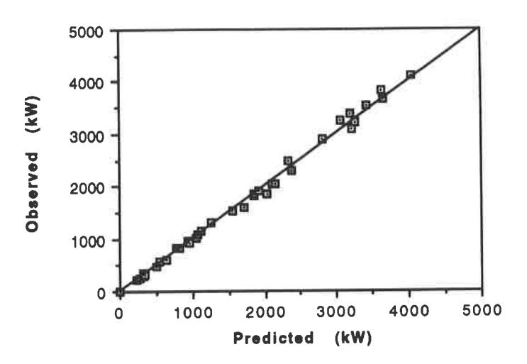
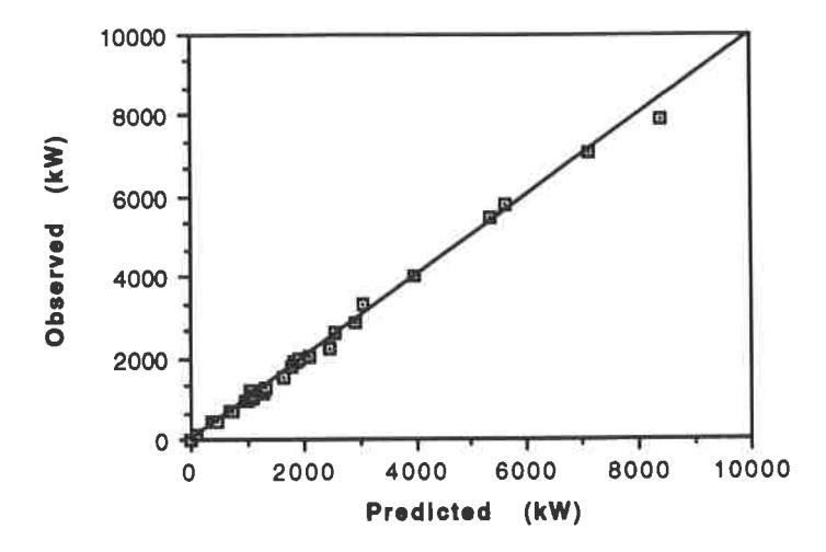
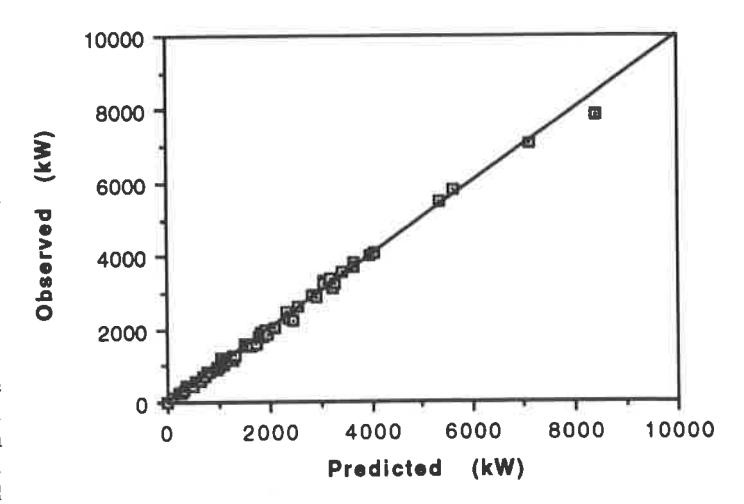
To determine whether the power model was able to accurately predict the power draw of mills, the model's calibration constant (k) was fitted to the database and its predictions of the individual mill's power draw determined. The results are shown graphically in Figures 4–6. The results for ball and AG/SAG mills are shown separately as well as in a combined form. It is emphasised, however, that the predictions derive from the one model which relates to all mills.
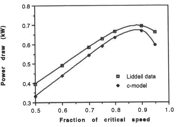
It can be seen that the predicted values agree well with the observed ones. Ideally, however, validation needs to be carried out on data independent of the database. Although from a laboratory mill, the data obtained by Liddell (1986) presented an opportunity to validate the C-model's response to changes in mill speed and load. Liddell used a 0.545 m diameter mill with a 0.308 m length. It was charged with steel balls and was run at a
range of speeds. For one of his series of tests the mill was charged with steel balls to a filling of 40 per cent. A sand/water slurry of 46 per cent solids content by volume was then added. The speed was varied in the range 50–95 per cent of critical and the power determined using a torque meter on the motor output shaft and the mill's rotational rate.
Liddell's data are shown in Figure 7 with the results from the C-model superimposed. The net power draw from the model is plotted as it is more likely to correspond to the measurement obtained by Liddell from his mill. This machine used a much simpler and, most likely, more efficient drive train than industrial mills against which the C-model was calibrated. In addition, the torque meter on Liddell's mill measured motor output power and hence did not include motor inefficiency. It is expected, therefore, that the net power of the C-model which is the power absorbed by the charge only, would be slightly lower than that measured by Liddell. From Figure 7 this is indeed the case. The C-model net power is consistently lower than that measured over the full range of speeds. The shape of the power curve is almost identical, however, indicating a realistic response of the model to changes in mill speed.
CONCLUSIONS
A mathematical model (C-model) of the power draw of tumbling mills has been developed which is based on the observed motion of the charge inside a glass laboratory mill. On the basis of a database 76 ball mill, SAG mill and AG mill data sets ranging in power draws from 6.8–7900 kW, this model was found to provide accurate predictions, with a relative precision of 10.6 per cent at the 95 per cent confidence level. In addition to the database, Liddell's data (1986) from a laboratory mill run at a wide range of speeds, was also used to validate the model. Good agreement was found.
While collecting data on mill dimensions, operating conditions and power draw it became apparent that in many cases these data are not measured with sufficient accuracy on plants. In addition, some operational staff were not fully aware of the power capability of their mills. To ensure full utilisation of plant it is essential that the mill design and operating limits are known.
ACKNOWLEDGEMENTS
The support of the sponsors of the AMIRA/JKMRC project P9K is gratefully acknowledged both financially and with regard to the free access to their milling plant which was provided.
REFERENCES
- Bond, F C, 1961. Crushing and grinding calculations. Allis Chalmers Publication No 07R9235B , Revised Jan.
- Bond, F C, 1962. Additions and revision to Crushing and grinding calculations (Bond, 1961).
- Harris, C C, Schnock E M and Arbiter N, 1985. Grinding mill power consumption, Mineral Processing and Technology Review, 1:297-345.
- Liddell, K S, 1986. The effect of mill speed, filling and pulp rheology on the dynamic behaviour of the load in a rotary grinding mill. MSc Thesis, University of Witwatersrand, Johannesburg, South Africa.
- Morrell, S, Johnson, G and Revy, T, 1991. A comparison through observation and simulation of the power utilization performance of two dissimilar comminution plants, in Proceedings 4th Mill Operators' Conference , Burnie, Tasmania, pp 157-160 (The Australasian Institute of Mining and Metallurgy: Melbourne).
- Morrell, S, 1992. Prediction of grinding mill power, Trans IMM , 101:C25-32.
- Morrell, S, 1993. The prediction of power draw in wet tumbling mills. PhD Thesis. University of Queensland, Australia.
- Taggart, A F, 1945. Handbook of Mineral Dressing (Wiley: New York).