



The content on this page was automatically generated from the PDF publication document and may contain errors or inaccuracies. Please refer to the original PDF for the most accurate information.
Power draw of wet tumbling mills and its relationship to charge dynamics—Part 1: a continuum approach to mathematical modelling of mill power draw
S. Morrell
Synopsis
A theoretical approach to the modelling of the power draw of industrial tumbling mills is described that is based on the motion of the grinding charge. The charge is treated as a continuum, which allows analytical solutions to the equations that are developed. The model is equally applicable to ball-, semi-autogenous and autogenous mills and contains a description of the power draw of both the cylindrical section and the cone-ends. Differences between the power draw of grate- and overflow-discharge mills are described from consideration of the different shapes and compositions of their charges. A large database of industrial mill data is used to demonstrate the accuracy of the model.
The rotation of a cylindrical tumbling mill moves the charge that it contains and in so doing consumes energy. Hence, the key to determining the rate at which this energy is consumed (the power draw) lies in being able to describe the motion of the charge. Taggart's comments1 in this regard are particularly relevant: 'Net power is not capable of analytic determination because of present ignorance of the internal dynamics of the tumbling load'. However, until recently little attention has been paid to developing models of the power draw of industrial grinding mills that explicitly contain a description of the dynamics of the charge. Notable exceptions have been the work of Lukasiewicz and co-workers2 and the discrete-element approach of Mishra and Rajamani,3 but, as is the case with other mill power models that can be found in the literature, 4-12 no comprehensive database is provided to validate them conclusively.
In the present two-part contribution an approach to the prediction of grinding mill power is described that satisfies the need for a description of the dynamics of the charge, yet, through the use of simplifying assumptions, results in models that are easy to use. In this first part a model, referred to as the 'C-model', of mill power draw is described that is based on measurements of the way the charge in a wet grinding mill moves. In the second part13 an empirical model, the 'E-model', is described that is based on the response of the C-model but which contains fewer and simpler equations. Full details of an extensive database of ball-, autogenous and semi-autogenous mills, together with their associated power draws, are provided. The accuracy of the models is illustrated with the use of this database.
General modelling approach
A model that treats the charge as a continuum (C-model) is described here in Part 1 of the contribution. The approach that is adopted in the model is to estimate the rate at which the mill shell provides potential and kinetic energy to the charge (i.e. the power draw due to motion of the charge) from a description of the shape and motion of the charge. The gross power draw is predicted by making allowances for the power consumption associated with motor and drive-train inefficiencies and with heat losses due to internal friction within the charge, together with the energy required for breakage by attrition/abrasion and for rotation of the grinding media. The model can be expressed as:
Gross power =
No-load power + \( (k \times \text{Charge-motion power}) \) (1)
where gross power is the power input to the motor (i.e. metered power); no-load power is the power input to the motor when the mill is empty; charge-motion power is the power associated with the movement of the charge; and \( (k \times \text{charge-motion power}) \) is the total power input to the charge = net power. k is a lumped parameter that allows for heat losses due to internal friction and the energy consumed by attrition/abrasion breakage and rotation of the grinding media, plus inaccuracies associated with measurements (and related assumptions) of the shape and motion of the charge.
The power associated with the motion of the charge is estimated by employing a mathematical description of the shape and position of the charge and of the velocities of particles within it. The data that are used to construct this description were obtained by inspection of photographs of the motion of a charge in a 0.3-m diameter glass-ended laboratory tumbling mill. The technique has been described in an earlier publication; 14 more recent research 15 has extended the range of rotational speeds investigated. In addition, whereas in the earlier work a smooth-lined mill was used, in the later research 5 mm high lifters were installed. Mill fillings in the range 15–45% of mill volume were tumbled in the laboratory mill in the speed range 73–112% of critical.
No-load power was used to estimate the drive-train and motor inefficiencies and is modelled using an empirical relationship that is based on data from industrial mills. The lumped parameter, k, was then determined by comparing the no-load and charge-motion power with the gross power draws, which were recorded during detailed surveys of the performance of a large number of full-scale mills.
Modelling of dynamics of charge
Charge shape
The resistance that the mill motor feels to its rotation, and,
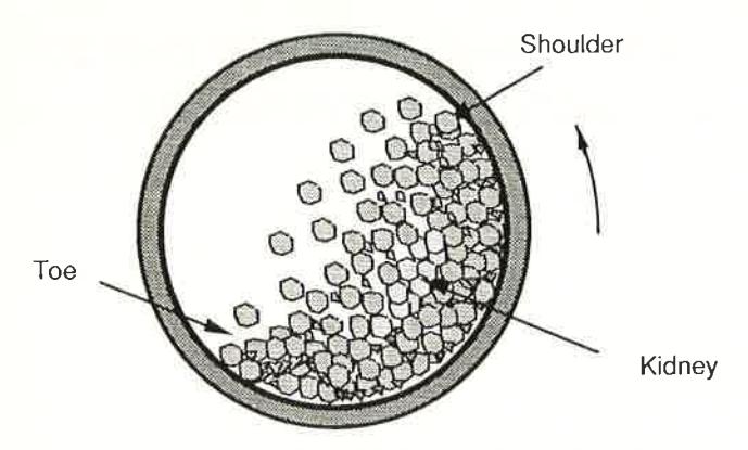
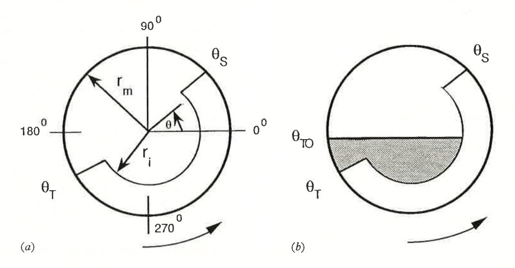
hence, its power draw, is caused only by that part of the charge which exerts a force on the mill shell, the part of the charge that is in free flight having no direct effect on the mill. Similarly, the material in the kidney (Fig. 1) has little effect. This can be inferred from measurements made on photographs of the mill charge. It is found that the volume of material in the kidney varies according to filling and speed conditions but is of the order of 3-6% of the total volume of the charge. Since this material is effectively stationary, has relatively small mass and lies quite near the centre of rotation of the mill, the associated power draw will be significantly less than 3-6% of the total. Therefore, those parts of the charge in free flight and in the kidney can be ignored with little effect on the accuracy of the model. The remainder of the grinding charge (hereafter called the 'active charge') forms a crescent-shaped mass, which is adequately approximated by Fig. 2(a)). These simplifications enable a description of the general shape of a mill charge that renders its mathematical treatment possible, yet at the same time reflects the essential shape that is observed in practice. The photographic evidence suggests that this shape is more appropriate than the flat, inclined surface that has been the basis of most grinding-mill power modelling over the past 30 years. 4-9 This approach, however, has been criticized by some authors for excluding the kidney material.5 In relation to the development of a relatively simple but accurate power draw model, the minimal effect on power draw that the kidney has renders this argument trivial.
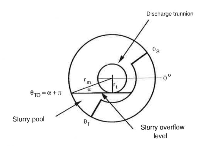
The condition represented in Fig. 2(a) typically reflects that found in grate-discharge mills. In such mills the charge normally runs with the interstices in the grinding media rarely filled much beyond the point where all the voidage is occupied by slurry. However, in an overflow-discharge mill slurry can only leave the mill when it overflows the discharge trunnion. Excess slurry is therefore present, giving rise to the second charge shape shown in Fig. 2(b). In this case a pool of slurry is present in addition to the grinding media. The slurry pool is assumed to comprise a mixture of ore and water of the same density as the discharge slurry. The remainder of the charge comprises the grinding media, whose interstices are fully occupied by slurry of the same density as the discharge slurry. Thus, the only difference between the overflow- and grate-discharge configurations is the presence of a slurry pool in the former. However, it should be noted that even in grate-discharge mills a slurry pool may develop as a result of insufficient grate and/or pulp-lifter capacity. The level of slurry will vary depending on the volumetric flow rate into the mill in relation to the grate/pulp-lifter capacity. 17
The boundaries of the grinding-media charge are defined by radii with angular displacements of \( \theta_S \) and \( \theta_T \) and their intersection with the mill shell and a circle that describes the boundary between the kidney and the active charge (Fig. 2(a)). The latter boundary has a radius \( r_i \) and is hereafter referred to as the inner surface of the charge. The angles \( \theta_S \) and \( \theta_T \) describe the locations of the points in the charge known, respectively, as the 'shoulder' and 'toe'.
Variation in positions of shoulder and toe
Measurements were made on the photographs taken in the laboratory glass mill of the angular displacement of the toe and shoulder \( (\theta_S \) and \( \theta_T) \) as the mill speed and filling were varied. The angular displacements were measured relative to zero degrees at the three o'clock position (see Fig. 2(a)). The results are plotted in Fig. 3, where it can be seen that the effect of increasing mill speed is to raise the charge higher and, hence, increase the shoulder angle. After leaving the mill shell at the shoulder the charge falls to the toe region, where it tends to accumulate while waiting for the mill to accelerate it to its rotational velocity. As a result, for a given mill filling the position of the toe appears not to vary over most of the speed range, confirming the results of Liddell and Moys. 18 Eventually, a speed is reached at which centrifuging begins. At this point the shoulder and, in particular, the toe angles tend rapidly to the 90° position. However, the entire charge does not begin to centrifuge at the same mill
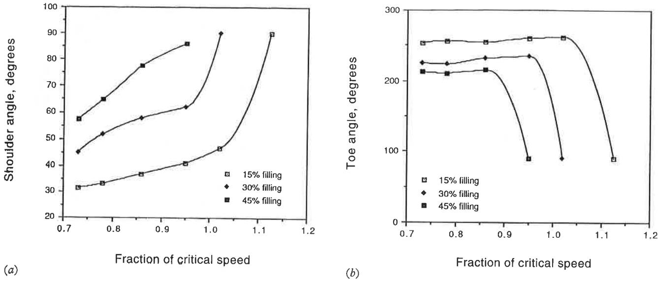
speed, the outer layers being the first to do so. Further increases in speed cause more and more layers to centrifuge until eventually the entire charge is centrifuging.
The mill filling is also seen from Fig. 3 to influence the positions of the toe and shoulder. Larger mill fillings give rise to higher shoulder angles and lower toe angles. As a result, the mill speed at which centrifuging commences is seen to be a strong function of the mill filling, higher fillings centrifuging at much lower speeds. This result is also in accordance with the findings of Liddell and Moys18 and is a departure from the view of a single centrifuging speed that is dictated solely by the balance of gravitational and centrifugal forces. In such an approach the effects of interaction are ignored. It is clear, however, that the charge behaves as a collective body and that interactions cannot be ignored. Thus, owing to the pressure exerted by the charge the material lower down the rising face of the mill helps support the material higher up the face and causes it to reach a higher position than would be the case with single particles moving inside the mill. With greater mill fillings the effect is more pronounced and gives rise to higher shoulder angles. This phenomenon is related to mill speed and the magnitude of the frictional forces within the charge. The latter forces are, in turn, directly proportional to the weight of the charge, 18,19 As the relative magnitude of these forces is independent of mill diameter, the relative position of the charge will be the same regardless of mill diameter provided that the mill filling and the percentage of critical speed remain constant,
Mathematical description of variation in toe and shoulder positions
To describe the variation in toe angle the following form of empirical equation was used:
$$ \theta_{\rm T} = A (1 - e^{-B(\phi_{\rm c} - \phi)}) + \frac{\pi}{2} $$ (2)
where \( \theta_T \) is toe angle, radians;* A and B are functions of the fractional mill filling, \( \mathcal{J}_t \) ; \( \phi \) is the fraction of the theoretical critical speed at which the mill is run; and \( \phi_c \) is the experi mentally determined fraction of the theoretical critical speed at which centrifuging is fully established (i.e. when most of the charge is centrifuging). \( \phi_c \) is also a function of \( \mathcal{J}_t \) of the form \( C + D\mathcal{J}_t \) , where C and D are constants.
To ensure that at centrifuging speed the angular displacement of the toe and shoulder converged to the same value ( \( \frac{\pi}{2} \) radians) the shoulder angle, \( \theta_S \) , was expressed as a function of \( \theta_T \) . The following form of equation was used:
$$ \theta_{S} $$ , radians = \( \frac{\pi}{2} - \left(\theta_{T} - \frac{\pi}{2}\right) \left(E + F\mathcal{J}_{t}\right) \) (3)
where E and F are functions of \( \phi \) .
The constants A, B, C, D, E and F were fitted to the data plotted in Fig. 3 by simple linear regression techniques, giving the relationships:
$$ \theta_{\rm T} = 2.5307 (1.2796 - \mathcal{J}_{\rm t}) (1 - e^{-19.42(\phi_{\rm c} - \phi)}) + \frac{\pi}{2} $$ (4)
where
$$ \phi_c = \phi; \ \phi > 0.35 (3.364 - \mathcal{J}_t) $$ (4a)
$$ \phi_c = 0.35 (3.364 - \mathcal{J}_t); \ \phi \le 0.35 (3.364 - \mathcal{J}_t) $$ (4b)
and
$$ \times [(0.3386 + 0.1041\phi) + (1.54 - 2.5673\phi) \mathcal{I}_{\uparrow}] $$ (5)
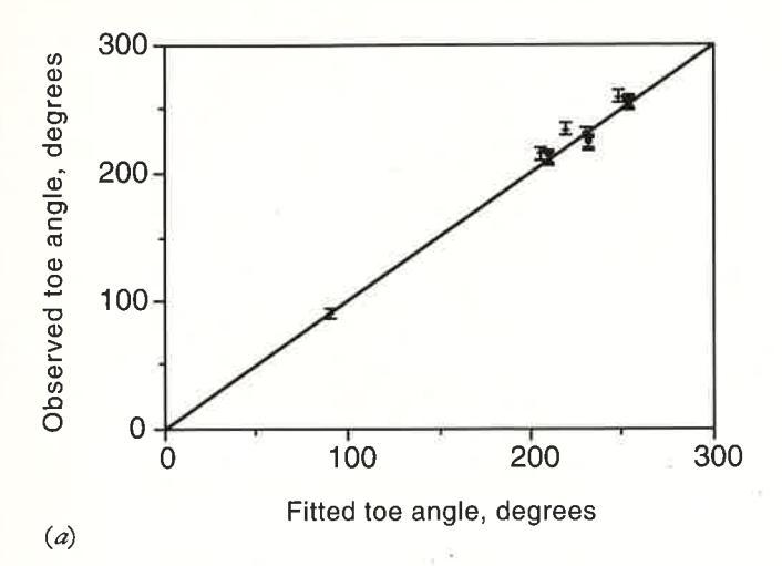
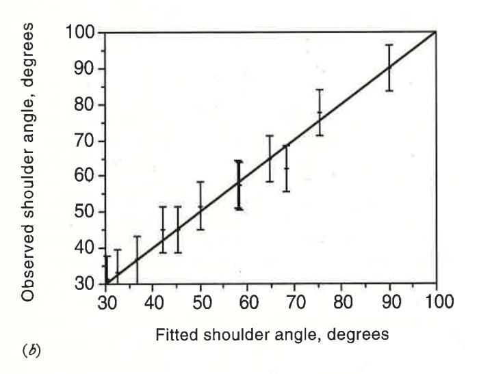
The fit of these equations to the observed data is shown graphically in Fig. 4, where measurement error bars associated with a 95% confidence interval are also displayed.
Motion of charge
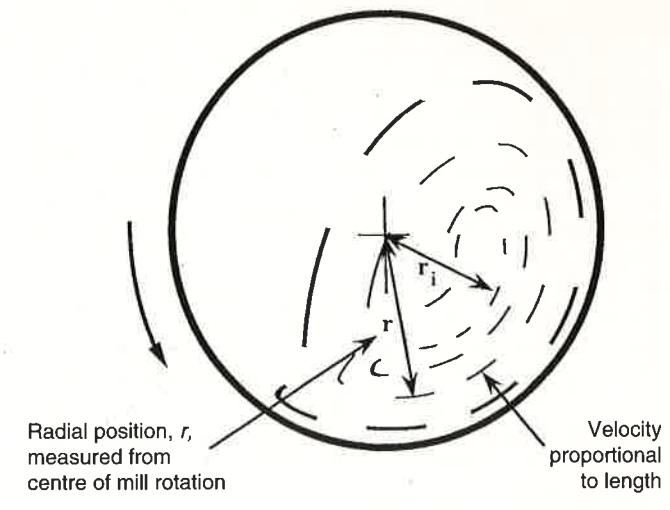
The velocity of particles in different parts of the charge was also determined from the photographs of the laboratory glass mill. With the use of brightly coloured tracers and a slow shutter speed the tracers appeared as lines of colour, the lengths of which were proportional to their velocity (Fig. 5).
* Symbols and their meanings are listed on page C52.
It was found that the particles in the active part of the charge described fairly concentric streamlines, the radial positions of which were measured along with their associated tangential velocities.
The velocities were normalized with respect to the speed of the mill shell. Similarly, the radial positions of streamlines were normalized with respect to the radius of the mill. Pairs of data were, thus, generated that comprised a normalized velocity, \( V_{\rm n} \) , and an associated normalized radial position, \( R_{\rm n} \) . Hence
and
where r is radial position, \( r_{\rm m} \) is mill radius at the wear face of the mill-shell liner, \( V_{\rm r} \) is tangential velocity at r and \( V_{\rm m} \) is tangential velocity of the wear face of the mill-shell liner.
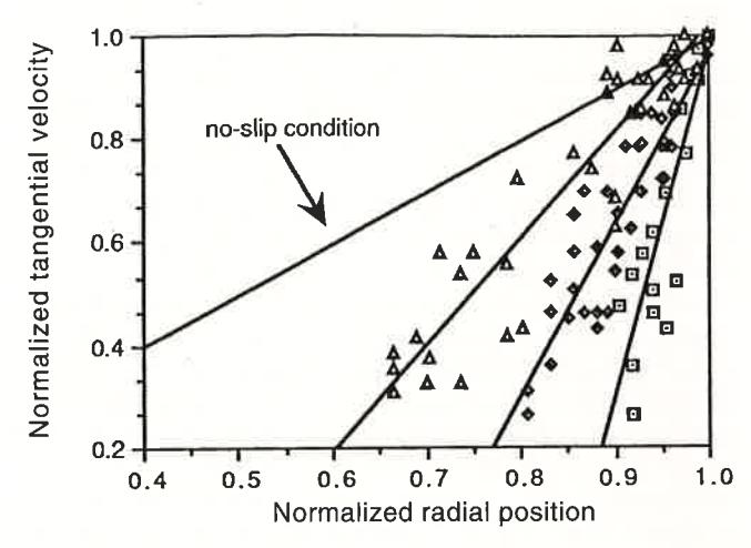
The data that were collected are plotted in Fig. 6. It can be seen that, despite some scatter, there is an approximately linear relationship between \( R_n \) and \( V_n \) , the gradient of which is dependent on the mill filling. The scatter is a result of the measurement technique that was employed, surging that occurred in varying degrees under all conditions and the variation in velocity along streamlines.20 The plots also show the relationship between tangential velocity and radial position under the assumption that the charge is fully locked ('no-slip' condition). It is apparent that an angular velocity gradient exists in the charge that is a function of mill filling. This is a direct result of the occurrence of slip within the charge. As the frictional force is proportional to the applied force acting in a direction normal to it, it is to be expected that the increased bed weights associated with larger mill fillings will generate greater frictional forces in the charge and, therefore, that less slip will occur within it. Hence, as the mill filling is increased the velocity gradient with respect to the mill radius will tend towards the no-slip condition.
Mathematical description of velocity profile
The tangential velocity, \( V_r \) , at a given radial position, r, can be expressed in terms of a rotational rate, \( N_r \) , by means of the equation
Through use of a simple linear relationship between the normalized tangential velocity and the normalized radial position, and by expressing velocity in terms of rotational rate, the following relationship was derived:
where \( r^* = zr_i \)
\( r_i \) is inner surface radius of the charge and \( r_m \) is mill radius.
From equation 9 \( r^* \) is the theoretical normalized radial position at which \( N_r = 0 \) . This position was related to the inner surface radius of the charge, \( r_i \) , by the parameter z using measurements of the position of \( r_i \) that were made on photographs of the mill charge. The z parameter was found to be a function of the fractional mill filling, \( \mathcal{J}_t \) . Hence, from equations 9 and 9a it can be seen that as \( \mathcal{J}_t \) increases \( N_r \) tends to \( N_m \) —i.e. the no-slip condition is approached.
Power-draw equations
The approach that was adopted in the development of the model was to consider the rates at which potential and kinetic energy is provided to the charge. As power can be defined as energy per unit time, the rates at which potential and kinetic energy is provided to the charge will provide an estimate of the power draw of the mill.
With reference to Fig. 7, consider an element within the surface ABCD of length L and width dr. The area of the element is given by Ldr. The tangential velocity of particles travelling through this surface is \( V_r \) and, hence, the volumetric flow rate through the surface is \( V_rLdr \) and the mass flow rate is \( V_r\rho_cLdr \) .
The path of particles travelling through the element of surface is assumed to be as shown in Fig. 7. Thus, the rate at which potential energy is imparted to them is given by \( V_r \rho_c L drgh \) , where the height difference, h, is given by \( h = r(\sin\theta_S - \sin\theta_T) \) . The rate at which kinetic energy is imparted to the particles is given by \( (V_r^3 \rho_c L dr)/2 \) .
If it is assumed that none of the energy of particles passing through surface ABCD is subsequently recovered by the
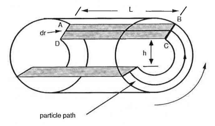
mill, the sum of the rates at which potential and kinetic energy is generated for all particles passing through surface ABCD, \( P_{r} \) , is given by
Also
Expressing \( V_r \) in terms of \( N_r \) therefore gives
$$ P_{t} = \int_{r_{i}}^{r_{m}} \left( 2\pi N_{r} r^{2} L \rho_{c} g(\sin \theta_{S} - \sin \theta_{T}) + \frac{(2\pi N_{r} r)^{3} L \rho_{c}}{2} \right) dr $$ (11)
From equation 9 the rotational rate, \( N_r \) , was related to the radial position, r, which allowed for the observed slip that occurred as r varied between \( r_{\rm m} \) and \( r_{\rm i} \) . Hence, substitution for \( N_r \) in equation 11 gives
$$ +\frac{4\pi^{3}L\rho_{c}N_{m}^{3}r_{m}^{3}}{(r_{m}-zr_{i})^{3}}\int_{r_{i}}^{r_{m}}(r-zr_{i})^{3}dr $$ (12)
Therefore
+ $$ L\rho_{c} \left( \frac{N_{m} r_{m} \pi}{(r_{m} - z r_{i})} \right)^{3} \left[ (r_{m} - z r_{i})^{4} - r_{i}^{4} (z - 1)^{4} \right] $$ (13)
Equation 13 was derived on the assumption that the charge has the shape shown in Fig. 2(a) and, hence, is applicable to grate-discharge mills. For overflow-discharge mills the effect of the slurry pool must be incorporated. The presence of the slurry pool results in a reduction of the power draw of the overflow mill relative to a grate-discharge unit of the same size. Such differences in power draw have been incorporated in an empirical manner in some mill-power equations. \( ^{6,14} \) Mechanistically, this effect can be considered to be caused by the buoyancy force to which the grinding charge is subject as it falls through the slurry pool. This part of its motion occurs between the surface of the pool and the toe of the grinding charge as defined by \( \theta_{\rm TO} \) and \( \theta_{\rm T} \) , respectively, and results in a reduction in the rate at which potential energy is imparted relative to the situation in a grate-discharge mill.
To incorporate this effect a buoyancy term was added to equation 13—resulting in the following single equation, which describes both grate and overflow mills:
$$ P_{t} = \frac{\pi g L N_{m} r_{m}}{3 (r_{m} - z r_{i})} \left[ 2 r_{m}^{3} - 3 z r_{m}^{2} r_{i} + r_{i}^{3} (3 z - 2) \right] \times $$ $$ \times \left[ \rho_{c} \left( \sin \theta_{S} - \sin \theta_{T} \right) + \rho_{p} \left( \sin \theta_{T} - \sin \theta_{TO} \right) \right] + $$ $$ + L \rho_{c} \left( \frac{N_{m} r_{m} \pi}{(r_{m} - z r_{i})} \right)^{3} \left[ \left( r_{m} - z r_{i} \right)^{4} - r_{i}^{4} (z - 1)^{4} \right] $$ (14)
where \( \rho_p \) is density of slurry, \( \rho_c \) is density of grinding charge, \( \theta_{TO} \) is angle of slurry pool (for grate-discharge mills \( \theta_{TO} = \theta_T \) ), \( \theta_S \) is given by equation 5 and \( \theta_T \) is given by equation 9.
The level of the slurry pool depends largely on the diameter of the discharge trunnion. A larger trunnion diameter will result in a lower slurry level, and vice versa. From simple geometry the angle of the slurry pool (Fig. 8) can be estimated from the equation
In the absence of data on the diameter of the trunnion it can be assumed that it is equal to one-quarter of the mill diameter. In this case \( \theta_{TO} = 3.395 \) .
Conical end-sections
Some mills, particularly those with large diameter to length ratios, are not completely cylindrical but have ends of conical form. The charge that moves in this section of the mill also
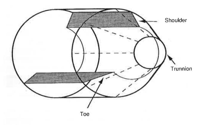
draws power and, hence, must be considered if the overall power draw of the mill is to be determined. The shape of the charge in such mills is assumed to be as shown in Fig. 9. For simplicity the shape is shown only for the grate-discharge mill.
It is assumed that the positions of the toe and shoulder are the same in the cone-ends as in the cylindrical section, but, owing to the keying effect of the end lifters, there is no angular velocity gradient in this part of the charge.
Using a similar approach to that adopted for the power draw of the cylindrical section, the following equation was derived for the combined power draw of the two conical end-sections:
$$ P_{c} = \frac{\pi L_{d}g N_{m}}{3(r_{m} - r_{t})} \left\{ \left( r_{m}^{4} - 4r_{m}r_{i}^{3} + 3r_{i}^{4} \right) \times \left[ \rho_{c} \left( \sin \theta_{S} - \sin \theta_{T} \right) + \rho_{p} \left( \sin \theta_{T} - \sin \theta_{TO} \right) \right] \right\} + \frac{2\pi^{3} N_{m}^{3} L_{d} \rho_{c}}{5(r_{m} - r_{t})} \left( r_{m}^{5} - 5r_{m}r_{i}^{4} + 4r_{i}^{5} \right) $$ (15)
A full derivation of equation 15 is given in Appendix 1.
Equations 14 and 15 constitute the two principal equations for calculating the power draws associated with the charge in the cylindrical and conical end-sections, respectively, of a wet tumbling mill. Apart from design parameters (such as the diameter and length, etc., of the mill) and the shoulder and toe angles, the equations contain three variables whose values must be known before the equations can be used. These are: \( r_i \) , the inner surface radius of the charge, \( \rho_c \) , the density of the charge, and \( \rho_p \) , the density of the pulp.
Radius of inner surface of charge, \( r_i \)
The inner surface of the charge defines the radial limit of the active part of the charge and it can be represented by its radial distance, \( r_i \) , from the axis of rotation. If the locations of the toe and shoulder are known, along with the volume of the charge between these points, \( r_i \) can be found from simple geometry:
where \( \beta \) is the active part of the charge expressed as a fraction of the total charge. This fraction will be proportional to the time that material spends in the active part of the charge relative to the time that it takes to complete one circuit of the entire charge. Hence
where \( t_c \) is mean time taken to travel between the toe and shoulder within the active part of the charge and \( t_f \) is mean time taken to travel between the shoulder and toe in free fall. \( t_c \) and \( t_f \) were approximated as follows:
where the mean rotational rate is
where the mean radial position, \( \overline{r} \) , is
$$ \bar{r} = \frac{r_{\rm m}}{2} \left[ 1 + \left( 1 - \frac{2\pi \mathcal{J}_{\rm t}}{2\pi + \theta_{\rm S} - \theta_{\rm T}} \right)^{0.5} \right] $$ (21)
By substituting equations 17-21 into equation \( 16 r_i \) can be estimated.
It should be noted that the fractional mill filling, \( \mathcal{J}_t \) , which was used to calculate \( r_i \) , is based on the cylindrical section. This radius is used to represent the location of the inner surface of the charge when the mill is in operation. If the mill has a conical ends, this surface extends into the cone-ends. Hence, the same value of \( r_i \) is also used in the calculation of cone-end power draw (see equation 15). Therefore, when conically ended mills are being considered \( \mathcal{J}_t \) still refers to the fractional mill filling in the cylindrical section only. No allowance needs to be made for the filling in the conesctions as this is automatically accounted for in the coneend power equation.
Charge and pulp density
The charge density, \( \rho_c \) , can be estimated from the equation14
where E is fractional porosity of charge; \( \rho_p \) is pulp density = fractional solids content (by volume) of discharge slurry; and U is fraction of grinding media voidage occupied by slurry.
U is fraction of grinding media voidage occupied by slurry. In the absence of data for E, \( \mathbf{v}_{\mathbf{p}} \) and U values of 0.4, 0.5 and 1, respectively, can be assumed. In this case equation 22 simplifies to
$$ \rho_{c} = 0.8 \rho_{o} + \frac{0.6 \mathcal{J}_{B} (\rho_{B} - \rho_{o})}{\mathcal{J}_{t}} + 0.2 $$ (23)
No-load power
To be practically useful a power model needs to predict accurately the gross (i.e. metered) power draw. The difference between gross and net power draw in a mill is due to losses associated with various electrical and mechanical components. The main losses occur in the motor, gearing and bearings. None of these remains constant over the mill's full operating range. Some, however, may have a fixed component—for example, losses in the bearings due to friction are dictated by the weight of the mill when empty (a fixed component, though even this will vary as liners and lifters wear) and the weight of the mill charge (a variable component). In most, if not all, full-scale operating plants
the only data that are measured are gross power and/or current and it is therefore not possible to measure directly the electrical and mechanical power losses. In rare cases the no-load power (the gross power drawn by the mill when running empty) is known from commissioning or maintenance records. Alternatively, if the mill has been emptied for relining, the no-load power is sometimes recorded at start-up. Such data indicate the magnitude of some of the components of the power loss.
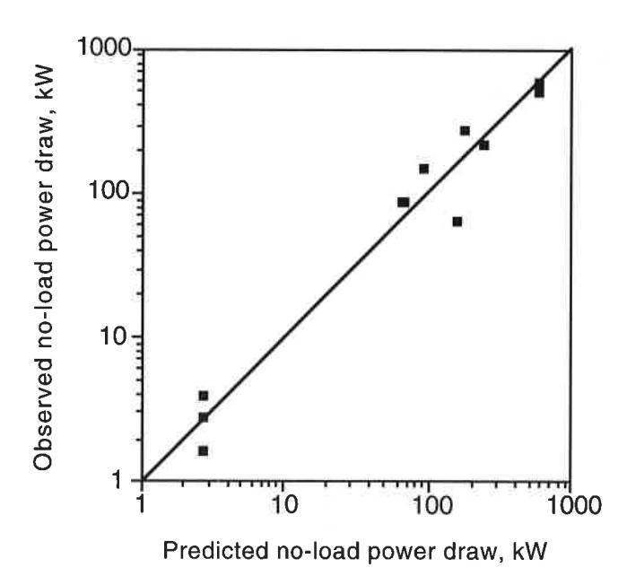
To determine the relationship between no-load power and mill design parameters ten data sets were analysed from nine mills with diameters ranging from 1.75 to 9.5 m. The following empirical relationship was developed:
No-load power, kW = $$ 1.68 D^{2.05} [\phi (0.667 L_d + L)]^{0.82} $$ (24)
where D is mill diameter, L is length of cylindrical section, \( L_{\rm d} \) is length of cone-end and \( \phi \) is fraction of critical speed.
A plot of the observed no-load power draws and of the predicted no-load power draws that were obtained with this equation is presented as Fig. 10. Scatter is apparent in the data and is attributed to differences in the mechanical design and condition of such components as bearings. This is illustrated by the data points for the lowest power draws, which represent readings taken from two different pilot mills with the same nominal dimensions.
Calibration and validation of model
Database
A total of 82 data sets were collected to calibrate and test the validity of the model. Details of the range of tumbling mills covered by the database are given in Table 1. Full details of the mills are given in Part 2 of the contribution.13
Calibration of model
Equations 14, 15 and 24, which contain no unknowns, can be used to estimate the no-load and charge-motion power requirements. This leaves the parameter k to be determined, after which equation 1 can be used to predict the gross power draw:
No-load power + $$ (k \times \text{Charge-motion power}) $$ (1)
Information for all the mills in the database was used to select a value of k that provides the best fit to the data. The resulting value of 1.26 implies that the energy consumed by sound, heat generated by sliding friction in the charge, attrition/abrasion breakage and rotation of the grinding media, along with a component arising from inaccuracies in the model, amounts on average to an additional 26% of the power draw due to the motion of the charge. This compares with estimates by Harris and co-workers8 of up to 20% and Rolf and Simonis21 figure of more than 30% for power associated with sliding motion.
Accuracy of model
The apparent accuracy of the model (with the above value for k) was evaluated from the standard deviation of the relative errors associated with predictions of the individual
| Ball-mills | Semi-autogenous mills |
Autogenous
mills |
||
|---|---|---|---|---|
| Diameter, m | 0.85-5.34 | 1.75-10.2 | 1.75-10.2 | |
| Belly length inside liners, m | 1.52-8.84 | 0.45-7.95 | 0.45-5.18 | |
| Length/diameter ratio | 1.00-1.83 | 0.33-1.50 | 0.33 - 1.0 | |
| Per cent of critical speed | 61-83 | 48-89 | 72-78 | |
| Ball filling, vol% | 20-48 | 3-25 | 0 | |
| Total filling, vol% | 20-48 | 7–38 | 10-31 | |
| Specific gravity of ore | 2.6-4.5 | 2.6 - 4.1 | 2.7 - 4.6 | |
| Number of mills | 40 | 23 | 6 | |
| Number of data sets | 43 | 31 | 8 | |
| Power draw, kW | 6.2-4100 | 10.4-10 013 | 9.3-8000 | |
| Relative error, % | ||
|---|---|---|
| Ball-mills | ||
| Mean | -0.4 | |
| Standard deviation | 5.4 | |
| 95% confidence interval | ±10.5 | |
| Autogenous/semi-autogenous mills | ||
| Mean | +0.4 | |
| Standard deviation | 9 | 4.6 |
| 95% confidence interval | ±9.0 | |
| All mills | ||
| Mean | < 0.1 | |
| Standard deviation | 5.0 | |
| 95% confidence interval | ±9.8 |
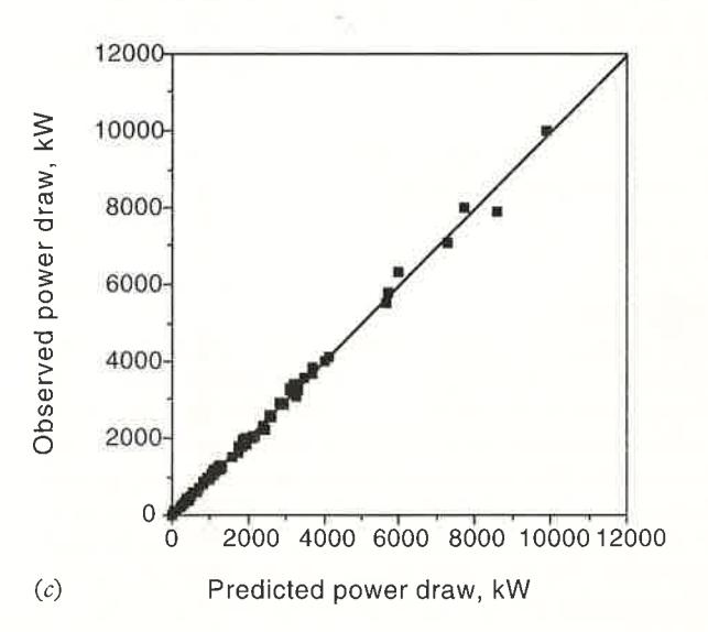
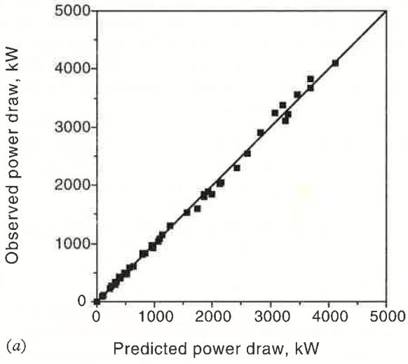
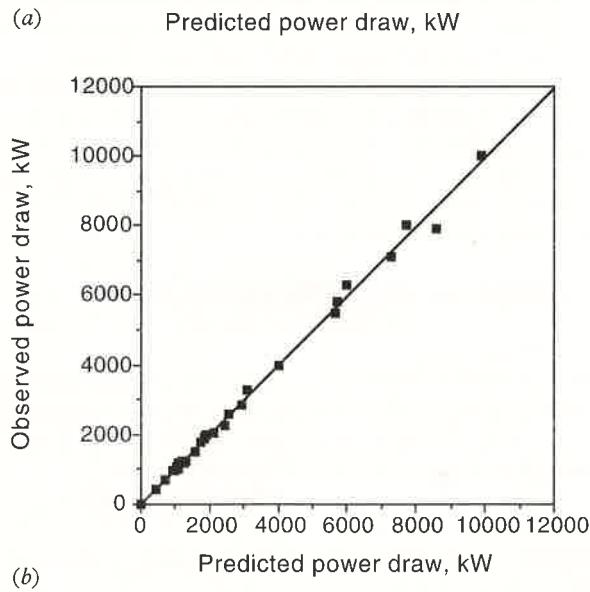
power draws of each of the mills in the database. The results, together with the 95% confidence interval, are given in Table 2. The overall standard deviation was 5.0%, giving rise to a 95% confidence interval of \( \pm 9.8\% \) . Graphically, the accuracy of the model is also illustrated in comparisons of the observed and predicted power draws in Fig. 11. It should be noted that, for illustrative purposes, the plots show the ball-mill and semi-autogenous/autogenous data separately as well as together. In all cases, however, the predictions of power draw were made with the same model, and a worked example is given in Appendix 2.
Validation of model
Given the size and diversity of the database, the good fit of the model predictions to the data is in itself confirmation that the C-model accurately predicts the power draw of industrial grinding mills. Ideally, however, validation needs to be carried out with independent data—i.e. with data other than those contained in the database. Although from a laboratory mill, the data obtained by Liddell22 present an opportunity to validate the response of the C-model to changes in mill speed and load. Liddell used a 0.545-m diameter mill with a length of 0.308 m. It was charged with steel balls and was run at a range of speeds. In one of his series of tests the mill was charged with steel balls to a filling of 40% and a slurry consisting of 46 vol% sand in water was then added. The speed was varied in the range 50-95% of critical and the power was determined from a torque meter on the motor output shaft and the mill's rotational rate.
Liddell's original data, less the no-load power of his mill (0.015 kW), are shown in Fig. 12 with the C-model's predictions of net power draw superimposed. Error bars associated with a 95% confidence level are also shown. It can be seen that the predictions of the model are particularly close to Liddell's data in the speed range 70–90% and that in all cases the observed data fall within the 95% confidence interval of the predictions.
Conclusions
A mathematical model (the C-model) of the power draw of tumbling mills has been developed that is based on the observed motion of the charge inside a glass laboratory mill. Comparison of the predictions of power consumption made by the model with information held in a database consisting of 82 data sets for ball-mills, semi-autogenous mills and
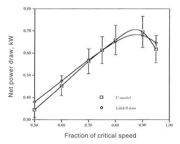
autogenous mills ranging in power draw from 6.2 to 10 000 kW showed the predictions to be accurate. Liddell's data22 for a laboratory mill that was run at a wide range of speeds were also used to validate the model. Good agreement was found
In Part 2 of the present contribution13 a much simpler empirical model is described whose performance is based on that of the C-model. In addition, full details of the mill database that was used to validate the models are provided.
Acknowledgement
The support of the sponsors of the AMIRA-JKMRC project P9K, both financially and in respect of the free access to their milling plant that was provided, is gratefully acknowledged.
References
- 1. Taggart A. F. Handbook of mineral dressing (New York: Wiley, 1945).
- 2. Lukasiewicz S. A. Swisterski W. and Romaniszyn G. Supercritical revolutions of tumbling mills. Mineral. Metall. Process. , 7, May 1990, 100-6.
- 3. Mishra B. K. and Rajamani R. K. Numerical simulation of charge motion in a ball mill. Preprints of the 7th European symposium on comminution , 1990, 555-63.
- 4. Arbiter N. and Harris C. C. Scale-up and dynamics of large grinding mills—a case study. Chapter 26 in Design and installation of comminution circuits Mular A. L. and Jergensen II. G. V. eds (New York: AIME, 1982), 491–505.
- 5. Austin L. G. A mill power equation for SAG mills. Mineral. Metall. Process. , 7, 1990, 57–63.
- 6. Bond F. C. Crushing and grinding calculations Allis Chalmers Publin no. 07R9235B, revised Jan. 1961.
- 7. Bond F. C. Additions and revision to Crushing and grinding calculations (reference 6), 1962.
- 8. Harris C. C. Schnock E. M. and Arbiter N. Grinding mill power consumption. Mineral Processing and Technology Review , 1, 1985, 297–345.
- 9. Hogg R. and Fuerstenau D. W. Power relationships for tumbling mills. Trans. SME-AIME , 252 , 1972, 418–23.
- 10. Moys M. H. A model for mill power as affected by mill speed, load volume and liner design. Reference 3, 595–607.
- 11. Rose H. E. and Evans D. E. The dynamics of the ball mill, part I: power requirements based on the ball and shell system. Proc. Inst. Mech. Engrs , 170 , 1956, 773–83.
- 12. Rose H. E. and Evans D. E. The dynamics of the ball mill, part II: the influence of the powder charge on power requirements. Proc. Inst. Mech. Engrs , 170 , 1956, 784–92.
- 13. Morrell S. Power draw of wet tumbling mills and its relationship to charge dynamics—Part 2: an empirical approach to modelling of mill power draw. Trans. Instn Min. Metall. (Sect. C: Mineral Process. Extr. Metall.) , 105, 1996, C54–62.
- 14. Morrell S. Prediction of grinding-mill power. Trans. Instn Min. Metall. (Sect. C: Mineral Process. Extr. Metall.) , 101, 1992, C25–32.
- 15. Morrell S. The prediction of power draw in wet tumbling mills. Ph.D. thesis, University of Queensland, Australia, 1993.
- 16. Cilliers J. J. et al. A method of investigating rod motion in a laboratory mill. Minerals Engng , 7, nos 5/6 1994, 533–49.
- 17. Morrell S. and Stephenson I. Slurry discharge capacity of autogenous and semi-autogenous mills and the effect of grate design. Int. J. Mineral Process. , 1996, in press.
- 18. Liddell K. S. and Moys M. H. The effect of mill speed and filling on the behaviour of the load in a rotary grinding mill. J. S. Afr. Inst. Min. Metall. , 88 , no. 2 1988, 49–57.
- 19. Vermeulen L. A. and Howat D. D. Effect of lifter bars on the motion of en-masse grinding media in milling. Int. J. Mineral Process +, 24 , 1988, 143–59.
- 20. Vermeulen L. A. and Howat D. D. Fluctuations in the slip of the grinding charge in rotary mills with smooth liners. Mintek Technical Memorandum , 1984. (Project no. 16082)
- 21. Rolf L. and Simonis W. Energy distribution in ball mills. Reference 3,543-554.
- 22. Liddell K. S. The effect of mill speed, filling and pulp rheology on the dynamic behaviour of the load in a rotary grinding mill. M.Sc. thesis, University of the Witwatersrand, 1986.
Symbols
- Diameter of cylindrical section of mill inside liners, m
- E Fractional porosity of charge
- g Acceleration due to gravity, m s-2
- \( \mathcal{J}_{B} \) Fraction of mill volume in cylindrical section occupied by balls (including voids)
- \( \mathcal{J}_{t} \) Fraction of mill volume in cylindrical section occupied by balls and coarse ore charge (including voids)
- k Lumped parameter used in calibration of model
- L Length of cylindrical section of mill inside liners, m
- \( L_c \) Length of cone-end, measured from cylindrical section, at radius \( r_c \)
- \( L_d \) Length of cone-end, m
- \( L_i \) Length of charge surface within cone-ends, m
- \( N_{\rm m} \) Rotational rate of mill, rev s-1
- \( N_r^{\text{in}} \) Rotational rate of particle at radial distance r, rev s-1
- Pt Theoretical power draw associated with motion of charge in cylindrical section, kW
- Pc Theoretical power draw associated with motion of charge in cone-ends, kW
- r Radial position, m
- r* Theoretical radial location in active charge at which velocity equals zero
- \( r_{\rm c} \) Radius of cone-end at distance \( L_{\rm c} \) from cylindrical section, m
- ri Radial location of inner surface of charge, m
- \( r_{\rm m} \) Radius of mill inside liners, m
- r. Radius of discharge trunnion, m
- \( R_n \) Normalized radial position; \( R_n = r/r_m \)
- S Fractional solids content (by volume) of discharge slurry
- \( t_{\rm c} \) Time taken to travel between toe and shoulder in active charge
- \( t_{\rm f} \) Time taken to travel between shoulder and toe in free flight
- U Fraction of grinding media voidage occupied by
- \( V_r \) Tangential velocity of particle at radial distance r, \( {\rm m}\,{\rm s}^{-1} \)
- \( V_{-} \) Tangential velocity of mill-shell inside liners, m s-1
- \( V_{\rm n} \) Normalized tangential velocity; \( V_{\rm n} = V_{\rm r}/V_{\rm m} \)
Greek
- β Fraction of total charge that is in active region
- Fraction of theoretical critical speed
- φc Fraction of theoretical critical speed at which centrifuging actually occurs
- \( \theta_S \) Angular displacement of shoulder location at mill shell, radians
- \( \theta_{\mathrm{T}} \) Angular displacement of toe location at mill shell, radians
- \( \theta_{TO} \) Angular displacement of surface of slurry pool at toe, radians
- \( \rho_c \) Density of total charge, t m-3
- \( \rho_o \) Density of ore, t m-3
- \( \rho_{\rm B} \) Density of steel balls, t m-3
- \( \rho_{\rm p} \) Density of discharge pulp, t m-3
Appendix 1
With reference to Fig. 1, for an element of length \( {\rm d}L_{\rm c} \) in the cone section the power-draw equation has the same form as for a cylindrical vessel (equation 11 of the main text).
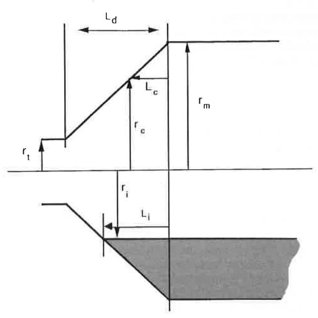
Hence, for the element of length \( \mathrm{d}L_\mathrm{c} \) at a cone radius of \( r_\mathrm{c} \) the power draw \( (P_{\mathrm{d}L_\mathrm{c}}) \) for a grate-discharge mill is given by
$$ P_{dL_{c}} = dL_{c} \int_{r_{i}}^{r_{c}} \left[ 2\pi N_{m} \rho_{c} r^{2} g \left( \sin \theta_{S} - \sin \theta_{T} \right) + 4\pi^{3} N_{m}^{3} r^{3} \rho_{c} \right] dr $$ (1)
As the radius of the cone varies with its length, for the entire cone equation 1 must be integrated with respect to the length of the cone, \( L_{\rm c} \) . Hence, the total power draw associated with both cone-ends, \( P_{\rm c} \) , is given by
$$ P_{c} = 2 \int_{0}^{L_{i}} \int_{r_{i}}^{r_{c}} \left[ 2\pi N_{m} \rho_{c} r^{2} g \left( \sin \theta_{S} - \sin \theta_{T} \right) + \left( 4\pi^{3} N_{m}^{3} r^{3} \rho_{c} \right) dr dL_{c} \right] $$ (2)
From geometry
Substitution of equation 4 into equation 2 gives
$$ P_{c} = \frac{2L_{d}}{(r_{m} - r_{t})} \left[ 2\pi N_{m} \rho_{c} g \left( \sin \theta_{S} - \sin \theta_{T} \right) \int_{r_{c}}^{r_{m}} \int_{r_{i}}^{r_{c}} r^{2} dr dr_{c} + 4\pi^{3} N_{m}^{3} \rho_{c} \int_{r_{c}}^{r_{m}} \int_{r_{c}}^{r_{c}} r^{3} dr dr_{c} \right] $$ (5)
$$ = \frac{2L_{\rm d}}{(r_{\rm m} - r_{\rm t})} \left[ \frac{1}{6} \pi N_{\rm m} \rho_{\rm c} g \left( \sin \theta_{\rm S} - \sin \theta_{\rm T} \right) \times \right. $$ $$ \left. \times \left( r_{\rm m}^4 - 4 r_{\rm m} r_{\rm i}^3 + 3 r_{\rm i}^4 \right) + \right. $$ $$ \left. + \frac{1}{5} \pi^3 N_{\rm m}^3 \rho_{\rm c} \left( r_{\rm m}^5 - 5 r_{\rm m} r_{\rm i}^4 + 4 r_{\rm i}^5 \right) \right] $$ (6)
Using the same approach as was adopted for the cylindrical section, equation 6 can be extended to encompass overflow mills. Hence
$$ P_{c} = \frac{\pi L_{d} g N_{m}}{3(r_{m} - r_{t})} \left\{ \left( r_{m}^{4} - 4r_{m} r_{i}^{3} + 3r_{i}^{4} \right) \times \left[ \rho_{c} \left( \sin \theta_{S} - \sin \theta_{T} \right) + \rho_{p} \left( \sin \theta_{T} - \sin \theta_{TO} \right) \right] \right\} + \frac{2\pi^{3} N_{m}^{3} L_{d} \rho_{c}}{5(r_{m} - r_{t})} \left( r_{m}^{5} - 5r_{m} r_{i}^{4} + 4r_{i}^{5} \right) $$ $$ (7) $$
Appendix 2
To illustrate the use of the C-model a worked example is given for a semi-autogenous mill. The equation numbers given in the calculation steps refer to the equations of the main text.
Model input data
To execute the model certain design and operating data are required. These are summarized in Table 1.
| Diameter inside liners, m | 8 |
|---|---|
| Belly length inside liners, m | 4 |
| Centre-line length inside liners, m | 6 |
| Trunnion diameter inside liners, m | 2 |
| Mill rotational speed, rev min -1 | 10.77 |
| Fraction of critical speed | 0.72 |
| Specific gravity of ore | 2.75 |
| Specific gravity of balls | 7.8 |
| Total fractional mill filling of cylindrical section | 0.35 |
| Ball fractional mill filling of cylindrical section | 0.10 |
| Solids content of discharge slurry, vol% | 45.9 |
| Discharge mechanism | Grate |
Calculation steps
1—Calculate charge density, \( \rho_c \) Input data: \( \rho_o = 2.75 \) ; \( \rho_B = 7.8 \) ; \( \mathcal{J}_t = 0.35 \) ; \( \mathcal{J}_B = 0.1 \) ; \( \rho_p = 0.495 \) Assume U = 1 and E = 0.4From equation 22: \( \rho_c = 3.237 \)
2—Calculate toe angle, \( \theta_{\rm T} \) , slurry toe angle, \( \theta_{\rm TO} \) , and shoulder angle, \( \theta_{\rm S} \)
Input data: \( \mathcal{J}_{t} = 0.35 \) ; \( \phi = 0.72 \)
From equation 4b: \( \phi_c = 1.0549 \)
From equation 4: \( \theta_T = 3.9198 \) radians
As the mill is a grate-discharge unit, \( \theta_{TO} = \theta_{T} \)
From equation 5: \( \theta_S = 0.8519 \) radians
3—Calculate inner surface radius of charge, r;
Input data: \( \mathcal{J}_t = 0.35 \) ; \( r_m = \text{mill diameter}/2 = 4 \text{ m} \) ; \( N_m = \text{(mill rotations per minute)}/60 = 0.179 \text{ rev s}^{-1} \)
From previous calculations: \( \theta_T = 3.9198 \) radians; \( \theta_S = 0.8519 \) radians
From equations 18 and 19: \( t_c = 5.7 \)
From equations 20 and 21: \( t_f = 0.926 \)
From equation 17: \( \beta = 0.856 \)
Then, from equation 16: \( r_i = 2.576 \)
4—Calculate z parameter
Input data: \( \mathcal{J}_t = 0.35 \)
From equation 9a: z = 0.8226
5—Calculate power draw due to motion of charge in cylindrical section, \( P_{\star} \)
Input data: \( \mathcal{J}_t = 0.35 \) ; \( r_m = \text{mill diameter}/2 = 4 \text{ m} \) ; \( N_m = (\text{mill rotations per minute})/60 = 0.179 \text{ rev s}^{-1} \) ; L = 4 m
From previous calculations: \( \theta_{\rm T} = 3.9198 \) radians; \( \theta_{\rm TO} = \theta_{\rm T} \) ; \( \theta_{\rm S} = 0.8519 \) radians; z = 0.8226; \( r_{\rm i} = 2.576 \) ; \( \rho_{\rm c} = 3.237 \) ; \( \rho_{\rm p} = 0.495 \)
Use \( g = 9.814 \text{ m s}^{-2} \)
From equation 14: \( P_{t} = 2809 \text{ kW} \)
6—Calculate cone-end charge-motion power, \( P_c \)
(It should be noted that the fractional mill filling, \( \mathcal{J}_t \) , used in the previous calculation step is based on the cylindrical section. This is used to calculate where the inner surface of the charge is when the mill is in operation and is described by the radius \( r_i \) . If the mill is conically ended, this surface extends into the cone-ends. Hence, the same value of \( r_i \) is also used in the calculation of cone-end power draw (see equation 15). Therefore, when cone-ended mills are being considered \( \mathcal{J}_t \) still refers to the fractional mill filling in the cylindrical section only. No allowance need be made for the filling in the cone sections as this is automatically taken into account in the cone-end power equation.)
Input data: \( r_{\rm t} \) = 1 m; \( L_{\rm d} \) = (centre-line length – belly length)/2 = 1 m; (all other parameters required have been determined in calculation step 5)
From equation 15: \( P_c = 378 \text{ kW} \)
7—Calculate no-load power
Input data: D = 8 m; \( \phi = 0.72 \) ; L = 4 m; \( L_d = 1 \text{ m} \)
From equation 24: no-load power = 322 kW
8—Calculate gross power
Total power draw due to charge motion in the cylindrical section and cone-ends = \( P_t + P_c = 3187 \) kW
No-load power = 322 kW
Calibration factor, k = 1.26
From equation 1: gross power = no-load power + \( (k \times \text{charge-motion power}) = 4338 \text{ kW} \)
The calculation steps for a ball-mill are identical to those given above. For most ball-mills the total fractional mill filling should be set to the same value as the ball fractional mill filling—i.e. \( \mathcal{J}_t = \mathcal{J}_B \) . This is equivalent to assuming that the rock charge occupies the voidage in the ball charge without causing significant dilatation of the ball bed. However, in some primary ball-mills in which coarse feed is being ground some dilatation may occur. In these cases allowance must be made by making \( \mathcal{J}_t \) greater than \( \mathcal{J}_B \) . In addition, where the mill is an overflow-discharge unit and the diameter of the discharge trunnion is known the slurry pool angle, \( \theta_{TO} \) , must be calculated using equation 14a. If the diameter of the discharge trunnion is not known, \( \theta_{TO} \) should be set to 3.395 radians.