



The content on this page was automatically generated from the PDF publication document and may contain errors or inaccuracies. Please refer to the original PDF for the most accurate information.
Power draw of wet tumbling mills and its relationship to charge dynamics—Part 2: an empirical approach to modelling of mill power draw
S. Morrell
Synopsis
Part 1 of this two-part contribution presented a mathematical model, based on the dynamics of the charge and termed the 'C-model', for prediction of the power draw of tumbling mills. Part 2 describes a simpler, empirical model (the 'E-model') whose performance is based on that of the C-model. The database of industrial ball-, semi-autogenous and fully autogenous mills that was collected for the validation of both models is described in detail. The database is used to assess the predictive capabilities of the E-model, showing it to be only slightly less accurate than the C-model despite its much simpler structure.
The author is not aware of any work published this century that presents a model (in the form of an equation or set of equations) of the power draw of a wide range of industrial grinding mills under a wide range of operating conditions with convincing attendant evidence of its ability to make accurate predictions. This lack of relevant experimental data has limited the practical application of many of the attempts that have been made to model the power draw of mills. Data on the power draw of grinding mills are abundant in the literature, but, as Harris and co-workers1 remarked, they are "... too frequently unusable simply because one or more essential variables have been omitted'. The absence of published results obtained from vigorous experimental testing of the various models has led to a general lack of evaluation of the validity of the assumptions and hypotheses that underlie such models. Harris and co-workers1 did make some effort to evaluate the performance of various power prediction equations and, in so doing, developed further a semiempirical equation of their own. However, since they used manufacturers' published data, which themselves were undoubtedly generated by proprietary equations of unproven validity, their equation remains unproven. To ensure that the models that are described in the two parts of the present contribution have a proven ability to predict accurately the power draw of industrial mills an extensive database was assembled. This part of the contribution provides full details of the database, which is used to validate the accuracy of a relatively simple empirical model—the E-model—whose performance is based on that of the C-model described in Part 1.2
Collection of grinding-mill data
Although small laboratory mills provide an excellent test-bed to determine the functional relationships between operating conditions and power draw, good-quality data for full-scale plant are required to determine whether such relationships hold at the industrial level.
The literature contains some data for industrial mills, but these are isolated cases and often lack sufficient detail to be useful for research purposes. The problem is compounded by the inherent difficulties in obtaining accurate data. In 1988 the author therefore began to assemble a database on grinding mills that could be used with confidence to develop and validate models of power draw.
The minimum details of a grinding mill that are required to enable prediction of its power consumption are: diameter (inside liners); length (inside liners); rotational speed; ball filling; total filling (balls plus rock); discharge mechanism (grate or overflow); and specific gravity of the ore.
Details of these parameters, as well as of the true power draw, were sought for as wide a range as possible of mill dimensions, ore types and operating conditions. During the course of their collection a variety of potential sources of error were encountered, and these are described in the next sections.
Mill diameter
The required mill diameter is that measured inside the liners rather than inside the shell. However, the diameter changes as the liners wear. Inside-liner diameters can only be reliably obtained by direct measurement from inside the mill at the time of recording the power draw. With a number of mills the author was able to do this. In some instances inside-shell diameters only were available and, in such cases, twice the nominal thickness of the half-worn liner was subtracted from the inside-shell diameter.
Mill length
Manufacturers often quote an 'effective grinding length' (EGL) for a mill, but it is apparent that manufacturers differ in their definition of what this is. In some cases it appears to be the length of the mill at the belly (i.e. the cylindrical section) inside the shell. In mills with conical ends this is misleading as it effectively ignores the volume of the mill within the ends. Some manufacturers take this into account by specifying an EGL that is between the belly length and the length along the centre-line. In such cases it has not been established how this length is determined. Whenever possible engineering drawings were sought and both belly and centre-line lengths were determined. In other cases direct measurement was possible. If neither of these was feasible, the manufacturer's EGL was used. As with the measurement of diameter, allowances were made for the thickness of the liners.
Mill speed
The most common method for reporting the rotational speed of the mill is as a percentage of the critical speed. This figure is often based on the number of revolutions of the mill in one minute and a nominal inside-liner dimension. As the percentage of critical speed is proportional to \( D^{0.5} \) , the value that is calculated using the true inside-liner dimension will differ from this value.* Whenever possible the rotational speed, rev min-1, was recorded and the percentage of critical speed at the inside of the liners was then calculated.
Specific gravity of ore and balls
Different grades of steel and different manufacturing techniques result in balls of varying specific gravities. Since no information was sought on the specific gravity of balls during the course of this research, a mean value of 7.8 has been used. In semi-autogenous grinding (SAG) and autogenous grinding (AG) mills, in particular, the specific gravity of the ore has a significant effect on the density of the charge and, hence, power draw. In all the data sets held in the database the mean specific gravity of the feed ore has been used. It is possible, however, that when blends of ore are being treated a harder constituent may be present with a specific gravity that differs from that of the rest of the ore. In such circumstances the specific gravity of the ore in the mill will be different from that of the feed ore.
Mill filling
The mill filling, or volume of charge in the mill, has a significant effect on the power draw. In ball-mills the filling remains fairly steady over time as it consists mainly of steel balls. It is common practice for operators to charge ball-mills with steel balls according to a power set-point. Owing to the very stable power draws that are usually seen with ball-mills, this procedure ensures that the mill is always charged to approximately the same level. Where direct measurements of the ball filling were not possible at the time when power readings were taken historical plant records were used as a source of ball filling data. However, in AG and SAG mills the feed ore contributes significant quantities of rock to the grinding media. As a result, changes in the size distribution and hardness of the feed ore will affect the quantity of ore in the mill and, hence, the power draw. In all cases direct measurements of the loads were made. With AG and SAG mills this entailed running the mills under steady-state conditions and then crash-stopping them under load. Whenever possible the mill was then entered through the feed trunnion and measurements of the width of the charge were taken in three places, together with inside-liner dimensions. From these measurements the volume of the load was calculated by simple geometry. In a number of cases access to the interior of the mill was denied. In these instances photographs were taken of the charge against the grate and the level of the charge was determined from engineering drawings of the grate and simple geometry. Alternatively, a rod was inserted into the mill to measure the level of the charge below the feed trunnion.
SAG-mill operations presented additional difficulties because of the ball filling, which, being mixed with the ore charge, was difficult to estimate. In most cases mills were allowed to grind out and the ball filling was then measured. However, owing to the damage that this procedure can cause to the liners/lifters, this was not always possible. In such cases operators' estimates had to be used.
Power draw
Plants vary widely in the type and complexity of their instrumentation. As a result, data on power draw were available from a range of devices, including kilowatt-hour meters, power transducers and ammeters. If more than one source of power data was available at a particular site, a check was made on whether all sources gave similar readings. If they did not, electrical staff at the plant were requested to investigate and correct the differences. In the event that this did not prove possible the data were not included in the database. If only one source of power measurement was available, efforts were made to ensure that independent checks of the accuracy of the power reading were made either prior to the field study or shortly afterwards.
Details of database
Ball-mills
Data were collected from 40 different mills, yielding a total of 43 data sets (see Table 1 of Appendix 1). Power draws vary from 6.2 to 4100 kW, with a corresponding range of diameters from 0.85 to 5.34 m. The majority of the mills were of the overflow type, only three relatively small mills in the power range 97–420 kW being grate-discharge. The speed range of the mills covered by the database ranges from 61 to 83% of critical. Most, however, are in the range 70–75% of critical.
Mill fillings were typically in the range 30–40%, though values as high as 48% and as low as 20% were recorded. Apart from one set of data for a pilot mill, most of the data for low fillings relate to very large-diameter mills (>4.8 m).
SAG mills
Thirty-one sets of data obtained from 23 SAG mills (Table 2 of Appendix 1) are held in the database. Diameters vary from 1.75 to 10.20 m, with a corresponding power-draw range of 10.4–10 000 kW. The large-diameter unit also has one of the largest ball loads (16%) recorded in the database, although its total filling was only 19%. Ball loads varied considerably from 3 to 25%, with a mean of 12%.
The speeds of the SAG mills varied from as low as 48% up to 89% of critical, with a mean of 75%. The low-speed mill was fitted with a variable-speed drive and was operated at this low speed specifically to generate data for the research programme. The high-speed mill is in a South African gold plant.
Included in the SAG mill database are four mills for which the masses of both the ore and the ball charge were measured by dumping their contents and weighing them. Three of the mills were full-size units with dimensions (diameter \( \times \) length) of 5.08 m \( \times \) 6.82 m, 7.05 m \( \times \) 3.66 m (see earlier work³) and 4.16 m \( \times \) 4.78 m, the data for the last mill being kindly provided to the author by Pendreigh.⁴ In addition to the full-size mills, data were obtained for a pilot unit.
AG mills
Autogenous mills are the least represented in the database (eight data sets), reflecting their less common use than SAG mills (Table 3 of Appendix 1). Despite this, the range of diameters that was covered in the fieldwork programme matched that of the SAG mills (1.75–10.2 m). The power range, however, was slightly smaller (9.3–8000 kW). Included were two mills whose entire equilibrium contents were weighed and sized—one a pilot unit and the other a unit with dimensions of 5.105 m \( \times \) 5.181 m. \( ^5 \)
* Symbols and their meanings are listed on page C59.
Empirical power-draw model
The availability of the database provided an opportunity to develop an empirical model that is based on the performance of the C-model2 but is of much simpler form. From the analysis of the factors affecting power draw that have so far been considered the following variables can be listed as influential: diameter, D; length, L; speed (fraction of critical), \( \phi \) ; charge density, \( \rho_c \) ; and mill filling, \( \mathcal{J}_{\tau} \) .
From analysis of the C-model equations the underlying relationships between these variables and power draw can be expressed in the following simple form, which is similar to that proposed by Harris and co-workers:1
Net power draw = $$ KD^{2.5}L_{o}\rho_{c}\alpha\delta $$ (1)
where \( \alpha \) and \( \delta \) are non-linear functions of filling and speed, respectively, D is mill diameter, \( L_{\rm e} \) is effective grinding length, \( \rho_{\rm c} \) is charge density and K is a calibration constant whose value depends on whether the mill has a grate or overflow discharge and which lumps together all other parameters and errors.
The rotational speed and mill filling are related in a complex manner to power draw owing to their influence on the positions of the toe and shoulder of the charge. Hence, to determine the functions \( \alpha \) and \( \delta \) the response of the C-model to both filling and speed was modelled empirically. In addition, the effective length of the mill was defined to take into account the effect of any cone-ends.
Effect of mill filling on power draw
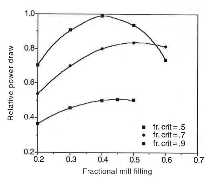
Fig. 1 illustrates the response of the C-model to changes in mill filling for a range of mill speeds. The power-draw data have been normalized with respect to the maximum power such that the power is in the range 0–1. It is seen that the filling at which power draw reaches a maximum ( \( \mathcal{J}_{max} \) ) is a function of mill speed, as was observed by Liddell. The values of \( \mathcal{J}_{max} \) for the speed range 50–100% of critical were determined iteratively from the C-model, and the results are given in Table 1.
From the data in Table 1 \( \mathcal{I}_{max} \) can be represented as a function of \( \phi \) by means of the polynomial expression
It appears from Fig. 1 that the relationship of power draw to mill filling is approximately parabolic and, hence, that it can be expressed as
Power $$ \propto \mathcal{J}_{t}(\omega - \mathcal{J}_{t}) $$ (3)
Differentiating power draw with respect to \( \mathcal{J}_t \) and setting to zero the filling at which power is a maximum gives the following expression for \( \mathcal{J}_{max} \) :
In models such as Bond's7,8 and Austin's9 \( \omega \) is a constant with a value close to unity—which gives, incorrectly, an invariant power maximum at a mill filling of around 50% (i.e. \( \mathcal{F}_{max} \approx 0.5 \) ). It is evident from Table 1 that \( \mathcal{F}_{max} \) (and \( \omega \) ) is, in fact, a function of mill speed. From equations 2 and 4 \( \omega \) can be represented as
| Fraction of critical speed, \( \phi \) | Filling at maximum net power, \( J_{\rm max} \) |
|---|---|
| 0.5 | 0.455 |
| 0.6 | 0.492 |
| 0.7 | 0.506 |
| 0.75 | 0.501 |
| 0.8 | 0.490 |
| 0.9 | 0.412 |
| 0.95 | 0.346 |
| 1.0 | 0.274 |
If the function \( \mathcal{J}_{t}(\omega - \mathcal{J}_{t}) \) is expressed as
then, from equations 4 and 6, the maximum value of \( \alpha \) is given by
To ensure that the expression given as equation 6 maintained values in a convenient range regardless of mill speed it was normalized with respect to \( \alpha_{max} \) . Hence, the equation was rewritten as
Effect of mill speed on power draw
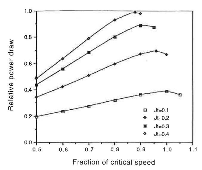
As with mill filling, the power draw reaches a maximum at a certain mill speed, above which it reduces. This effect is illustrated in Fig. 2, where the response of the C-model to mill speed is plotted. It is seen that for most of the speed range the response is approximately linear and that it only deviates from linear as the speed at which the power draw reaches a maximum is reached. This speed, \( \phi_{\text{max}} \) , is a function of the mill filling. This can be seen from Table 2,
| Fractional mill filling, \( J_{\rm t} \) | Fraction of critical speed at maximum net power, \( \phi_{max} \) | \( \phi^*_{\mathbf{max}} \) | |
|---|---|---|---|
| 0.1 | 1.00 | 0.9405 | |
| 0.2 | 0.96 | 0.9270 | |
| 0.3 | 0.92 | 0.9135 | |
| 0.4 | 0.88 | 0.9000 | |
| 0.5 | 0.84 | 0.8865 | |
where values of \( \mathcal{J}_t \) and associated values of \( \phi_{max} \) , as predicted by the C-model, are given.
To provide a speed function, \( \delta \) , that represented the speed trends exhibited by the C-model the following expression was used:
$$ \delta = \phi (1 - (1 - \phi_{\text{max}}^*) e^{-A(\phi_{\text{max}}^* - \phi)}) $$ (9)
where A is a constant and \( \phi^*_{\text{max}} \) is related to \( \phi_{\text{max}} \) (see below). This form provides a linear response over much of the speed range but allows a rapid reduction in power draw above a certain speed. Equation 9 has a form similar to Bond's speed function, which can be arranged as
Bond speed function = $$ \phi(1 - [1 - 0.9][2^{-10(0.9 - \phi)}]) $$
(9a)
The form of equation 9 was derived from that used to describe the position of the toe (see Part \( 1^2 \) ):
$$ \theta_{\rm T} = 2.5307 (1.2796 - \mathcal{J}_{\rm t}) (1 - e^{-19.42 (\phi_{\rm c} - \phi)}) + \frac{\pi}{2} $$ (10)
The exponential form of this equation gives a relatively small change in the toe angle over most of the range of mill speed. At elevated speeds, however, the angle of the toe changes rapidly as the charge begins to centrifuge. It is this movement of the toe that dominates the power-draw response of the mill to speed and, as a result, the power begins to fall. Equation 9 provides a similar response to changes in speed. The constant A in equation 9 was therefore assumed to take the same value as in the exponential term in equation 10 and was set at 19.42. The parameter \( \phi_{\text{max}}^* \) was then adjusted until equation 9 predicted the values of \( \phi_{\text{max}} \) listed in Table 2. The resulting values of \( \phi_{\text{max}}^* \) are also given in Table 2. They were found to be simply related to \( \mathcal{F}_1 \) by the equation
Effective grinding length
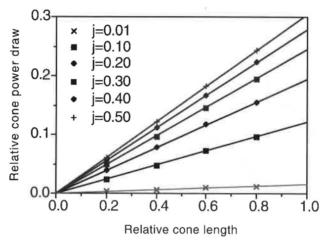
The effect of having conical end-sections in a mill is to increase the volume of the grinding chamber and, hence, the power draw relative to that of the cylindrical section alone. As the mill filling in the cylindrical section of the mill varies, the length of the cone-ends that is actively in use will also vary. Thus, as the mill filling increases the active or effective length of the cone-ends increases and, hence, so will the amount of power that the cone-ends draw relative to the cylindrical section. It follows from this that the so-called 'effective grinding length' (EGL) is not invariant but is a function of mill filling. To illustrate this effect the C-model was used to calculate the power draw of the cone-ends as a function of the length of the cones and the mill filling of the cylindrical section. The results are shown in Fig. 3, where the power draw and length of the cone-end are expressed relative to those of the cylindrical section (the power draw and length of the cone-end relate to the sum of both coneends). The geometries of the cones at each end were the same, with feed- and discharge-trunnion diameters equal to 0.25 of the mill diameter. It can be seen from Fig. 3 that the fraction of power draw attributable to the cone-end increases linearly with increasing cone length. The rate of increase, however, is a strong function of the mill filling of the cylindrical section.
The relationships illustrated in Fig. 3 were modelled by the equation
where \( P_{\rm cone-rel} \) is the ratio of the power draw of both coneends to that of the cylindrical section and \( L_{\rm cone-rel} \) is the ratio of the length of both cone-ends to that of the cylindrical section. Equation 12 can now be incorporated into an expression for an effective grinding length as follows:
where \( L_{\rm e} \) is effective grinding length, \( L_{\rm d} \) is mean length of the cone-ends (i.e. \( 0.5 \times \) (centre-line length – cylindrical section length)), L is length of the cylindrical section and \( \mathcal{J}_{\rm t} \) is fractional mill filling of the cylindrical section.
Calibration of empirical model
The empirical model (E-model) can now be written as
Gross power, kW = No-load power + $$ (KD^{2.5}L_{\rm e}\rho_{\rm c}\alpha\delta) $$ (14)
where
No-load power = $$ 1.68 D^{2.05} [\phi (0.667 L_d + L)]^{0.82} $$ (15)
$$ \delta = \phi (1 - [1 - \phi_{\text{max}}^*] e^{-19.42(\phi_{\text{max}}^* - \phi)}) $$ (18)
$$ \rho_{c} = \frac{\mathcal{I}_{t}\rho_{0}(1 - E + EU\rho_{p}) + \mathcal{I}_{B}(\rho_{B} - \rho_{0})(1 - E)}{\mathcal{I}_{t}} + \frac{\mathcal{I}_{t}EU(1 - \rho_{p})}{\mathcal{I}_{t}} $$ $$ (21) $$
and K is the calibration constant.
The difference between the power draws of grate- and overflow-discharge mills was related in Part \( 1^2 \) to the presence in the latter of a slurry pool. In the C-model the effect of this pool was incorporated by calculating the buoyancy force that it exerted on the charge. In the E-model the effect is incorporated in an empirical manner by fitting K to grate and overflow mills independently. For overflow mills K was found to be 7.98, whereas for grate mills the value is 9.10. The ratio of the two calibration factors is 1.14, which almost exactly matches Bond's correction factor for grate-discharge mills.
Accuracy of model
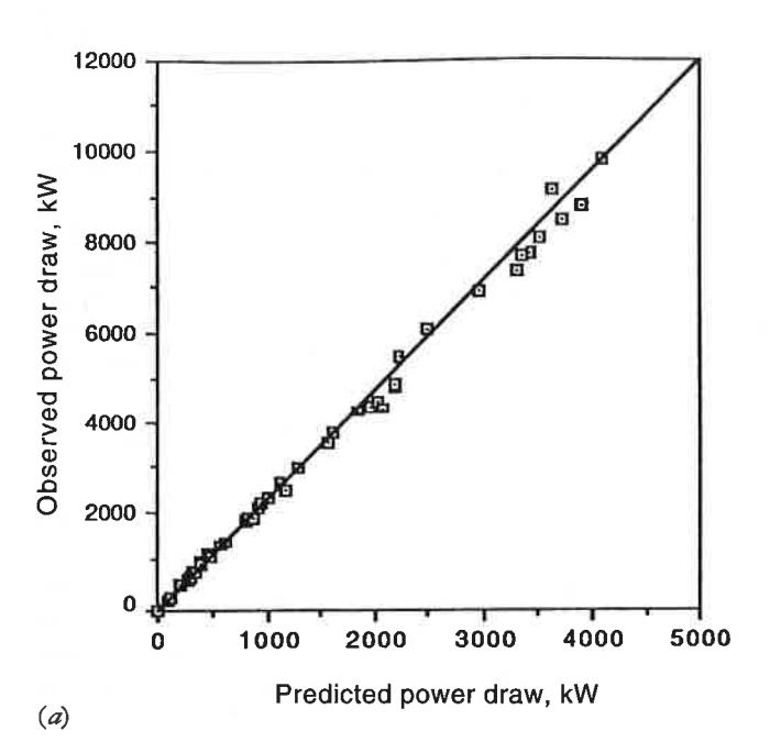
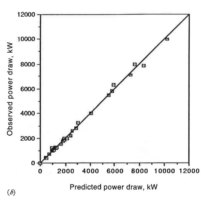
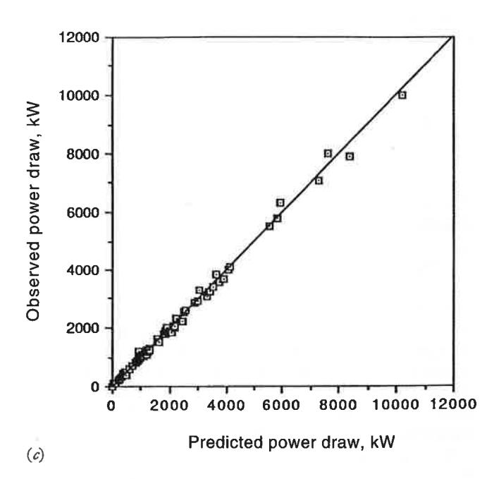
The mean relative error and standard deviation of the
|
Relative error, %
E-model |
C-mode | |
|---|---|---|
| Ball-mills | ||
| Mean | <0.1 | -0.4 |
| Standard deviation | 5.8 | 5.4 |
| 95% confidence interval | 11.3 | 10.5 |
| AG/SAG mills | ||
| Mean | +0.5 | +0.4 |
| Standard deviation | 6.6 | 4.6 |
| 95% confidence interval | 12.9 | 9.0 |
| All mills | ||
| Mean | -0.2 | < 0.1 |
| Standard deviation | 6.2 | 5.0 |
| 95% confidence interval | 12.1 | 9.8 |
Conclusions
By incorporating a description of the shape and motion of the charge a mathematical model (termed the 'C-model') was developed to predict the power draw of wet tumbling mills. Comparison with operational data held in a large and comprehensive database that covers AG, SAG and ball-mills in the power range 6.2–10 000 kW demonstrated that the model provides a high degree of accuracy. It was shown to predict the observed interaction between speed and mill filling in the power-draw response of the mills6 as well as the differences between the power draws of grate-discharge and overflow-discharge mills.7
By empirically describing the response of the C-model a much simpler model, the E-model, was developed and was found to be only marginally less accurate. Both models can easily be incorporated into a spreadsheet. Their operation can be checked using the worked examples provided in the appendices to Parts 1 and 2 and can be validated by reference to the database of industrial mills that is described in detail in this part of the contribution.
The successful ability of the C-model to predict accurately the power draw of such a wide range of mills is attributable in part to the incorporation of a description of the dynamics of the charge and vindicates comments that were made by Taggart 50 years ago. 10 However, the way in which the charge dynamics are described need not be complex. This was shown in the development of the E-model, which is empirically based on the response of the C-model yet suffers very little in its ability to make accurate predictions of power draw.
It is concluded that the models that have been described in Parts 1 and 2, together with the detailed data that were used to validate them, overcome the shortcomings of previous attempts to predict the power draw of mills accurately.
Acknowledgement
The support, both financial and in respect of the free access to their milling plant that was provided by the sponsors of the AMIRA-JKMRC project P9K, is gratefully acknowledged.
References
1. Harris C. C. Schnock E. M. and Arbiter N. Grinding mill power consumption. Mineral Processing and Technology Review , 1, 1985, 297–345.
- 2. Morrell S. Power draw of wet tumbling mills and its relationship to charge dynamics—Part 1: a continuum approach to mathematical modelling of mill power draw. Trans. Instn Min. Metall. (Sect. C: Mineral Process. Extr. Metall.), 105, 1996, C43–53.
- 3. Morrell S. Simulations of bauxite grinding in a semi-autogenous mill and DSM screen circuit. M.Eng. thesis, University of Oueensland, 1989.
- 4. Pendreigh R. Personal communication, 1991.
- 5. Stanley G. G. The autogenous mill—a mathematical model derived from pilot and industrial scale experiment. Ph.D. thesis, University of Queensland, 1974.
- 6. Liddell K. S. The effect of mill speed, filling and pulp rheology on the dynamic behaviour of the load in a rotary grinding mill. M.Sc. thesis, University of the Witwatersrand, 1986.
- 7. Bond F. C. Crushing and grinding calculations Allis Chalmers Publin no. 07R9235B, revised Jan. 1961.
- 8. Bond F. C. Additions and revision to Crushing and grinding calculations (reference 7), 1962.
- 9. Austin L. G. A mill power equation for SAG mills. Minerals Metall. Process. , 7, 1990, 57-63.
- 10. Taggart A. F. Handbook of mineral dressing (New York: Wiley,
Symbols
- D Diameter of cylindrical section of mill inside liners, m
- E Fractional porosity of charge
- \( \mathcal{J}_{B} \) Fraction of mill volume occupied by balls (including voids)
- Fraction of mill volume occupied by balls and coarse ore charge (including voids)
- K Lumped parameter used in calibration of model
- L Length of cylindrical section of mill inside liners, m
- \( L_{\rm c} \) Length of cone-end, measured from cylindrical section, at radius of \( r_{\rm c} \)
- \( L_{\rm d} \) Length of cone-end, m
- L Effective grinding length, m
- S Fractional solids content (by volume) of discharge
- U Fraction of grinding media voidage occupied by slurry
Greek
- α, ω Empirical parameters
- φ Fraction of critical speed
- \( \phi_{max}^* \) Fraction of critical speed at which power draw is maximum
- \( \theta_{\mathrm{T}} \) Angular displacement of toe position at mill shell, radians
- \( \rho_c \) Density of total charge, t m-3
- \( \rho_0 \) Density of ore, t m-3
- On Density of steel balls, t m-3
Author
S. Morrell graduated from the Royal School of Mines, London, England, in 1980 with a B.Sc.(Eng.) in metallurgy before taking up employment with De Beers in South West Africa and Botswana, where he worked in the areas of production, plant design and commissioning. In 1987 he joined the Julius Kruttschnitt Mineral Research Centre, University of Queensland, Australia, as a research scholar. After obtaining the degree of M.Eng. in 1989 he joined the staff of the research centre and is currently a project leader. In 1993 he gained a Ph.D. and was awarded the Zinc Corporation Prize for his work on mill power modelling.
Address: Julius Kruttschnitt Mineral Research Centre, Isles Road, Indooroopilly, Queensland 4068, Australia.
Appendix 1—Mill database
|
Discharge
mechanism |
Inside-liner
Diameter |
dimensions,
Belly length |
m
Centre-line length |
Mill speed
Rev min -1 |
% Critical |
Mill filling
Balls, % |
Total, % |
Ore
specific gravity |
Gross
power, kW |
|---|---|---|---|---|---|---|---|---|---|
| Overflow | 5.34 | 8.69 | 8.69 | 13.36 | 73 | 28 | 28 | 3.2 | 3669.0 |
| Overflow | 5.34 | 8.69 | 8.69 | 13.36 | 73 | 26 | 26 | 3.2 | 3549.0 |
| Overflow | 5.34 | 8.69 | 8.69 | 13.36 | 73 | 24 | 24 | 3.2 | 3385.0 |
| Overflow | 5.34 | 8.69 | 8.69 | 13.36 | 73 | 23 | 23 | 3.2 | 3251.0 |
| Overflow | 5.33 | 8.54 | 8.54 | 13.23 | 72 | 34 | 34 | 2.6 | 4100.0 |
| Overflow | 5.29 | 7.32 | 7.32 | 12.87 | 70 | 40 | 40 | 3.2 | 3828.0 |
| Overflow | 4.87 | 8.84 | 8.84 | 14.37 | 75 | 30 | 30 | 2.6 | 3225.0 |
| Overflow | 4.87 | 8.84 | 8.84 | 13.80 | 72 | 27 | 27 | 2.6 | 2900.0 |
| Overflow | 4.87 | 8.80 | 8.80 | 14.37 | 75 | 30 | 30 | 2.6 | 3104.0 |
| Overflow | 4.85 | 5.92 | 5.92 | 14.02 | 73 | 41 | 41 | 2.9 | 2550.0 |
| Overflow | 4.75 | 6.26 | 6.26 | 14.94 | 77 | 28 | 28 | 2.68 | 2050.0 |
| Overflow | 4.73 | 7.01 | 7.01 | 11.76 | 61 | 32 | 32 | 2.8 | 1840.0 |
| Overflow | 4.68 | 5.64 | 5.64 | 14.08 | 72 | 48 | 48 | 2.8 | 2300.0 |
| Overflow | 4.41 | 6.10 | 6.10 | 14.88 | 74 | 35 | 35 | 4.1 | 1900.0 |
| Overflow | 4.38 | 7.45 | 7.45 | 15.16 | 75 | 30 | 30 | 2.7 | 2026.0 |
| Overflow | 4.35 | 6.56 | 6.56 | 14.19 | 70 | 38 | 38 | 2.72 | 1850.0 |
| Overflow | 4.12 | 7.04 | 7.04 | 14.69 | 71 | 38 | 38 | 2.6 | 1800.0 |
| Overflow | 4.12 | 5.49 | 5.49 | 15.57 | 75 | 45 | 45 | 2.7 | 1600.0 |
| Overflow | 4.10 | 5.92 | 5.92 | 15.67 | 75 | 34 | 34 | 3.1 | 1525.0 |
| Overflow | 3.87 | 6.34 | 6.34 | 14.83 | 69 | 27 | 27 | 3.57 | 1075.0 |
| Overflow | 3.85 | 5.90 | 5.90 | 16.60 | 77 | 30 | 30 | 2.8 | 1300.0 |
| Overflow | 3.83 | 4.83 | 4.88 | 13.55 | 63 | 31 | 31 | 2.6 | 842.0 |
| Overflow | 3.55 | 4.87 | 4.87 | 16.16 | 72 | 40 | 40 | 2.8 | 970.0 |
| Overflow | 3.54 | 4.88 | 4.88 | 17.20 | 77 | 42 | 42 | 2.7 | 1029.0 |
| Overflow | 3.50 | 4.75 | 4.75 | 16.95 | 75 | 41 | 41 | 2.8 | 921.0 |
| Overflow | 3.50 | 4.42 | 4.42 | 16.73 | 74 | 35 | 35 | 2.75 | 820.0 |
| Overflow | 3.48 | 6.33 | 6.33 | 17.00 | 75 | 34 | 34 | 2.7 | 1150.0 |
| Overflow | 3.48 | 4.62 | 4.62 | 16.10 | 71 | 39 | 39 | 2.7 | 834.0 |
| Overflow | 3.05 | 4.27 | 4.27 | 17.68 | 73 | 45 | 45 | 3.9 | 600.0 |
| Overflow | 3.05 | 4.27 | 4.27 | 16.95 | 70 | 40 | 40 | 4.5 | 580.0 |
| Overflow | 3.04 | 3.05 | 3.05 | 19.77 | 82 | 45 | 45 | 3.5 | 475.0 |
| Overflow | 2.70 | 4.83 | 4.83 | 18.79 | 73 | 37 | 38 | 2.65 | 499.0 |
| Overflow | 2.70 | 3.40 | 3.40 | 20.08 | 77 | 36 | 36 | 2.7 | 334.0 |
| 2.64 | 3.66 | 3.66 | 18.22 | 70 | 43 | 43 | 2.8 | 420.0 | |
|
Grate
Overflow |
2.64 | 4.57 | 4.57 | 19.67 |
70
75 |
34 | 34 | 2.65 | 420.0 |
| 3.70 | 3.70 | 18.10 | 69 | 40 | 40 | 4.5 | 347.0 | ||
|
Overflow
Overflow |
2.60
2.52 |
3.66 | 3.66 | 17.98 | 68 | 35 | 35 | 2.7 | 265.0 |
| 4.20 | 82 | 36 | 36 | 2.7 | 299.0 | ||||
| Overflow | 2.30 | 4.20 | 22.87 | 235.0 | |||||
| Overflow | 2.29 | 2.74 | 2.74 | 23.11 | 83 | 44 | 44 | 3.5 | 97.0 |
| Grate | 1.73 | 2.44 | 2.44 | 22.03 | 69 | 35 | 35 |
2.7
2.7 |
103.0 |
| Grate | 1.70 | 2.70 | 2.70 | 26.27 | 81 | 40 | 40 | 103.0 | |
|
Overflow
Overflow |
0.85
0.85 |
1.52
1.52 |
1.52
1.52 |
32.57
32.57 |
71
71 |
40
20 |
40
20 |
2.9
2.9 |
6.2 |
| Mean | 3.68 | 5.53 | 5.54 | 17.18 | 73.12 | 35 | 35 | 2.98 | 1489.8 |
| Minimum | 0.85 | 1.52 | 1.52 | 11.76 | 61 | 20 | 20 | 2,60 | 6.2 |
| Maximum | 5.34 | 8.84 | 8.84 | 32.57 | 83 | 48 | 48 | 4.50 | 4100.0 |
|
Discharge
mechanism |
Inside-line
Diameter |
r dimensions,
Belly length |
m
Centre-line length |
Mill speed
Rev min -1 |
% Critical |
Mill filling
Balls, % |
Total, % |
Ore
specific gravity |
Gross
power, kW |
|---|---|---|---|---|---|---|---|---|---|
| Grate | 10.2 | 4.61 | 7.56 | 10.55 | 80 | 16 | 19 | 2.8 | 10013 |
| Grate | 9.59 | 4.27 | 5.86 | 10.24 | 75 | 19 | 31 | 2.6 | 7900.0 |
| Grate | 9.59 | 4.27 | 5.86 | 10.24 | 75 | 14 | 14 | 2.6 | 5790.0 |
| Grate | 9.59 | 4.27 | 5.86 | 10.09 | 74 | 19 | 19 | 2.6 | 7100.0 |
| Grate | 9.55 | 4.45 | 6.45 | 10.67 | 78 | 5 | 25 | 2.90 | 6300.0 |
| Grate | 8.38 | 3.26 | 5.00 | 11.69 | 80 | 14 | 18 | 2.65 | 4000.0 |
| Grate | 7.73 | 3.46 | 3.46 | 10.65 | 70 | 11 | 11 | 2.6 | 1800.0 |
| Grate | 7.23 | 3.00 | 3.00 | 11.80 | 75 | 11 | 16 | 2.72 | 1920.0 |
| Grate | 7.09 | 2.74 | 2.74 | 11.91 | 75 | 11 | 21 | 3.1 | 1900.0 |
| Grate | 7.05 | 3.66 | 3.66 | 11.23 | 71 | 12 | 31 | 2.65 | 2239.0 |
| Grate | 7.05 | 3.66 | 3.66 | 11.23 | 71 | 12 | 12 | 2.65 | 1500.0 |
| Grate | 6.51 | 2.44 | 2.44 | 11.77 | 71 | 3 | 16 | 4.1 | 972.0 |
| Grate | 6.50 | 2.42 | 3.02 | 12.44 | 75 | 6 | 21 | 3.64 | 1228.0 |
| Grate | 6.26 | 2.50 | 2.50 | 12.00 | 71 | 6 | 21 | 2.7 | 1200.0 |
| Grate | 5.82 | 5.65 | 5.65 | 14.20 | 81 | 13 | 33 | 2.8 | 2840.0 |
| Grate | 5.80 | 5.65 | 5.65 | 14.22 | 81 | 10 | 27 | 2.8 | 2600.0 |
| Grate | 5.30 | 7.95 | 7.95 | 13.04 | 71 | 18 | 30 | 2.8 | 3284.0 |
| Grate | 5.08 | 6.82 | 6.82 | 12.38 | 66 | 12 | 31 | 2.85 | 2000.0 |
| Grate | 5.05 | 5.99 | 5.99 | 14.49 | 77 | 17 | 21 | 2.68 | 2033.0 |
| Grate | 4.35 | 4.85 | 4.85 | 15.29 | 75 | 12 | 29 | 2.65 | 1066.0 |
| Grate | 4.16 | 4.78 | 4.68 | 18.45 | 89 | 10 | 38 | 2.7 | 1063.0 |
| Grate | 4.12 | 5.02 | 5.02 | 15.63 | 75 | 22 | 33 | 2.7 | 1225.0 |
| Grate | 4.12 | 5.02 | 5.02 | 15.63 | 75 | 22 | 22 | 2.7 | 1012.0 |
| Grate | 4.05 | 4.60 | 4.60 | 15.97 | 76 | 8 | 26 | 2.7 | 688.0 |
| Grate | 4.05 | 4.60 | 4.60 | 15.97 | 76 | 7 | 7 | 2.7 | 440.0 |
| Grate | 4.05 | 4.60 | 4.60 | 15.97 | 76 | 6 | 34 | 2.7 | 706.0 |
| Grate | 4.05 | 4.60 | 4.60 | 15.97 | 76 | 6 | 32 | 2.7 | 687.0 |
| Grate | 3.90 | 5.10 | 5.10 | 16.75 | 78 | 25 | 34 | 3.35 | 1175.0 |
| Grate | 3.85 | 5.69 | 5.69 | 10.35 | 48 | 12 | 12 | 2.8 | 404.0 |
| Grate | 1.75 | 0.45 | 0.64 | 24.94 | 78 | 8 | 23 | 2.65 | 11.0 |
| Grate | 1.75 | 0.45 | 0.64 | 24.94 | 78 | 4 | 24 | 2.65 | 10.4 |
| Mean | 5.92 | 4.22 | 4.62 | 13.89 | 74.75 | 12 | 24 | 2.81 | 2422.8 |
| Minimum | 1.75 | 0.45 | 0.64 | 10.09 | 48 | 3 | 7 | 2.60 | 10.4 |
| Maximum | 10.2 | 7.95 | 7.95 | 24.94 | 89 | 25 | 38 | 4.10 | 10013 |
|
Discharge
mechanism |
Inside-liner dimensions, m | Mill speed | Mill filling | Ore | Gross | ||||
|---|---|---|---|---|---|---|---|---|---|
| Diameter | Belly length | Centre-line length | Rev min -1 | % Critical | Balls, % | Total, % |
specific
gravity |
power,
kW |
|
| Grate | 10.20 | 4.73 | 7.18 | 10.06 | 76 | 0 | 26 | 3.6 | 8000.0 |
| Grate | 9.50 | 4.45 | 6.45 | 10.70 | 78 | 0 | 31 | 2.90 | 5490.0 |
| Grate | 7.10 | 2.43 | 3.47 | 11.43 | 72 | 0 | 12 | 4.6 | 1009.0 |
| Grate | 7.10 | 2.43 | 3.47 | 11.43 | 72 | 0 | 10 | 3.57 | 703.0 |
| Grate | 6.49 | 2.25 | 2.48 | 12.45 | 75 | 0 | 27 | 4 | 1240.0 |
| Grate | 6.49 | 2.25 | 2.48 | 12.45 | 75 | 0 | 19 | 4 | 960.0 |
| Grate | 5.11 | 5.18 | 5.18 | 13.63 | 73 | 0 | 24 | 4.2 | 1264.0 |
| Grate | 1.75 | 0.45 | 0.64 | 24.94 | 78 | 0 | 28 | 2.65 | 9.3 |
| Mean | 6.72 | 3.02 | 3.92 | 13.39 | 74.89 | 0 | 22 | 3.69 | 2334.4 |
| Minimum | 1.75 | 0.45 | 0.64 | 10.06 | 72 | 0 | 10 | 2.65 | 9.3 |
| Maximum | 10.20 | 5.18 | 7.18 | 24.94 | 78 | 0 | 31 | 4.60 | 8000.0 |
Appendix 2—Worked example
To illustrate the use of the E-model a worked example is given that relates to a SAG mill.
Input data
To execute the model certain design and operating data are required. These were summarized in Part 1 (Table 1 of Appendix 2, page C53).2
Calculation steps
1—Calculate charge density, \( \rho_c \) Input data: \( \rho_o = 2.75 \) ; \( \rho_B = 7.8 \) ; \( \mathcal{J}_t = 0.35 \) ; \( \mathcal{J}_B = 0.1 \) ; \( \rho_p = 0.495 \) Assume U = 1 and E = 0.4From equation 21: \( \rho_c = 3.237 \)
2—Calculate filling function, \( \alpha \) , and speed function, \( \delta \) Input data: \( \mathcal{J}_t = 0.35 \) ; \( \phi = 0.72 \) From equation 17: \( \omega = 1.02 \) From equation 16: \( \alpha = 0.225 \) From equation 19: \( \phi^*_{max} = 0.907 \) From equation 18: \( \delta = 0.718 \)
3—Calculate effective grinding length, \( L_{\rm e} \) Input data: \( {\cal J}_{\rm t}=0.35;~L=4;~L_{\rm d}= \) (centre-line length – belly length)/2 = 1 m From equation 20: \( L_{\rm e}=4.52 \) m
4—Calculate no-load power Input data: D=8 m; \( \phi=0.72 \) ; L=4 m; \( L_{\rm d}=1 \) m From equation 15: no-load power = 322 kW
5—Calculate gross power Input data: D=8 m From previous calculations: \( \rho_{\rm c}=3.237 \) ; \( L_{\rm e}=4.52 \) m; \( \alpha=0.225 \) ; \( \delta=0.718 \) ; no-load power = 322 kW Use K=9.1 for grate-discharge mills From equation 14: gross power = no-load power + \( (KD^{2.5}L_{\rm e}\rho_{\rm c}\alpha\delta)=4216 \) kW
The calculation steps for a ball-mill are identical to those given above. It should be noted that for ball-mills the total fractional mill filling should be set to the same value as the ball fractional mill filling—i.e. \( \mathcal{J}_t = \mathcal{J}_B \) . In addition, for overflow-discharge mills K = 7.98.