



The content on this page was automatically generated from the PDF publication document and may contain errors or inaccuracies. Please refer to the original PDF for the most accurate information.
The Application of Population Balance Models to Very Fine Grinding in Tower Mills
S Morrell1, U J Sterns2 and K R Weller2
ABSTRACT
Grinding to sizes less than 80 per cent passing 20 µm in both primary and regrind circuits is becoming increasingly important in processing metalliferous ores, as many of the remaining orebodies are very fine-grained and refractory. The process of very fine grinding, however, is expensive, and neither the performance nor the design criteria are well understood.
This paper presents some findings from a collaborative research program, one of the objectives of which has been to better understand and improve the performance of very fine grinding circuits. Data from surveys of an industrial tower mill grinding circuit are reviewed and analysed using the population balance models of the CSIRO and JKMRC. The performance of both models with regard to changes in feed size distribution, ball load and feedrate is assessed using these data.
From comparisons between pilot and full scale tower mill operation a prototype scaling methodology is also presented which shows promise in allowing the models to be used to predict the effect of changes in mill design.
INTRODUCTION
Grinding to less than an 80 per cent passing size ( \( P_{80} \) ) of 20 \( \mu \) m in both primary and regrind circuits is becoming increasingly important in processing metalliferous ores, as many deposits are known to be very fine-grained and refractory. Processing experience has shown that the energy cost of very fine grinding in traditional ball mills begins to rise exponentially as \( P_{80} \) falls below 75 \( \mu \) m, and 40 to 45 \( \mu \) m is seen by some to be the practical limit for ball mills. Several Australian companies have installed tower mills as one device which can offer a lower \( P_{80} \) and a significantly lower power draft. However, the effects of design and operating variables on performance criteria such as throughput, energy demand and size reduction have not been systematically quantified, so the limits to performance are difficult to predict.
This paper presents some findings from a collaborative research program, sponsored by a group of mining companies, an equipment company and one overseas research association. The work has been undertaken by groups from the Julius Kruttschnitt Mineral Research Centre (JKMRC), the CSIRO Division of Mineral and Process Engineering (CSIRO) and the University of South Australia. The program is co-ordinated by the Australian Mineral Industries Research Association (AMIRA). One of the objectives has been to better understand and improve the performance of tower mill grinding circuits.
In this paper, data from three surveys of an industrial tower mill circuit are analysed using the population balance and content based models developed for ball mills by the CSIRO and the JKMRC respectively, and results from both models are compared with experimental performance.
Data were also collected from a small pilot scale tower mill treating the same ore, and approximate breakage rates compared with the full scale results. A preliminary method of scaling up from pilot scale data is described and discussed.
- 1. JKMRC, Isles Road, Indooroopilly, Brisbane, Australia 4068.
- CSIRO Division of Mineral and Process Engineering, Pinjarra Hills, Qld, Australia 4000.
THEORY
The CSIRO form of the population balance model used for ball milling (Kelsall, Reid and Stewart, 1969; Austin, 1971) is a size-discrete, time-continuous first order rate model (Kelsall et al, 1969; Austin, 1971) based on a geometric size interval defined by a root-two testing sieve series. The breakage distribution function required to establish a size mass balance of the broken particles is assumed to be normal with respect to size and the same for all mineral components.
For continuous grinding under steady-state conditions, the rate-size mass balance around the mill for size i is given by:
$$ G_{pi} = G \text{ fi } - K_i H w_i + H \sum_{\substack{j=1\\i>1}}^{i-1} b_{i-j} k_j w_j $$ (1)
where G is the mass flow of solids through the mill, H is the mass of solids (excluding balls) held in the mill, \( f_i \) , \( p_i \) , \( w_i \) are the mass fractions of size i in the mill feed, product and hold-up respectively, \( k_i \) is the specific breakage rate constant and \( b_{i-j} \) the normalised breakage distribution function.
Dividing by the mass flow G gives:
$$ p_{i} = f_{i} - k_{i} \lambda w_{i} + \lambda \sum_{\substack{j=1 \ i>1}}^{i-1} b_{i-j} k_{j} w_{i} $$ (2)
where \( \lambda \) is the mean residence time of the solids in the mill.
The content based model used at the JKMRC (Whiten, 1974) is based on the same geometric size interval and is usually expressed as a rate-size mass balance of the mill contents as follows:
$$ 0 = Fi - ri Si + \sum_{j=1}^{i} a_{ij} r_{j} S_{j} - d_{i}S_{i} $$ (3a)
where \( F_i \) and \( P_i \) are the feed and product flow rates of size i, \( S_i \) is the total mass of size i held in the mill, \( r_i \) is the specific breakage rate constant, \( a_{ij} \) is the fraction of size j material which reports to the i size fraction after breakage, and \( d_i \) is the specific discharge rate.
From the definitions of both research groups \( P_i = Gp_i \) , \( F_i = Gf_i \) , \( S_i = Hw_i \) and \( r_i = k_i \) . It is also assumed that the breakage distribution (or appearance) function is normal with respect to size so \( a_{ij} \) Ü \( b_{i \cdot j} \) .
Making these substitutions in Equation 3a and 3b and combining them leads exactly to Equation 2 (but not the reverse). The notation of Equation 2 is carried forward in the paper.
In order to extract \( k_i \) values from Equation 2, given G, \( f^i \) and \( p_i \) , other measurements or assumptions must be made to determine H or \( \lambda \) , w and \( b_{i-j} \) .
Hold-up and residence time
The CSIRO approach is to measure the response of a mill (and classifier circuit when present) to an impulse of soluble tracer added to the mill feed. Weller (1981) has described how the overall mean residence time of the tracer in the mill (or circuit) is calculated from the concentration - time data gathered from the mill discharge, corrected when necessary, by the returns from a classifier. It is then assumed that the residence time of the tracer, water and all solids size fractions in the mill (not the circuit) are the same. This assumption allows \( \lambda \) and H to be estimated, assuming that the density of pulp held in the mill is the same as that in the mill discharge.
The problem now is to estimate \( w_i \) . Kelsall, Reid and Stewart (1969) and Weller (1981) have shown that the residence time distribution, measured from the impulse tracer data, can be closely fitted by one large and several equal small perfect mixers in series. The fitting yields two parameters; the fraction of hold-up in the big mixer (M) and the number of small mixers (N). As mixing is perfect, then by definition \( w_{iA} = p_{iA} \) where the subscript A refers to the first mixer. Using the product from one mixer as feed to the next effectively eliminates wi from Equation 2 and enables ki to be calculated. Once \( k_i \) is known, \( w_i \) of the total hold-up can be calculated from the \( p_{in} \) , N and \( M_n \) .
At the JKMRC, Whiten (1967, 1974, 1976) introduced the idea of a specific discharge rate di for size i such that:
The addition of Equation 4 allowed for the load related characteristics of grinding systems to be explicitly incorporated as well as providing a structure for describing the classifying effect in primary and grate discharge mills (Kavetsky and Whiten, 1982; Leung et al, 1987).
Using the definitions noted above, Equation 4 becomes:
$$ G_{pi} = d_i Hw_i \text{ or } d_i = p_i/(\lambda w_i) $$ (5)
Substituting in (2) to eliminate wi produces:
$$ p_{i} = f_{i} - \frac{k_{i}}{d_{i}} p_{i} + \sum_{\substack{j=1\\i>1}}^{i-1} b_{i-j} k_{j} p_{j} / d_{j} $$ (6)
leaving \( k_i/d_i \) as a function to be determined.
JKMRC practice for ball mills treating all but relatively coarse feed, is to use a single mixer and quote \( (k_i/d_i) \) as a single parameter, which is equivalent to reporting the CSIRO \( k_i \) values based on a single perfect mixer.
The residence time changes which result from a change in mill volume are introduced into the JKMRC model by arguing that solids hold-up is proportional to mill volume and hence the mean residence time will be a function of the volumetric feedrate. This is expressed as:
where
V volumetric feedrate
D mill diameter
L mill length
d* - normal discharge rate which should be near unity and constant (with respect to i) for no classification of the discharge.
The breakage rate parameter (ki/di) can therefore be defined as:
For a given set of feed and product data the breakage rate discharge parameter \( k_i/d_i \) can be back-calculated using Equation 6, providing \( a_{ij} \) is known. From Equation 8 the normal breakage parameter \( (k_i/d_i) \) can be calculated. The \( k_i/d_i \) values should remain constant regardless of mill dimensions and volumetric feedrate, providing the breakage and discharge are typical of the entire mill contents. This will always occur if the mill is perfectly mixed and is approximated in many other cases. When simulating changes in feedrate or changes in mill volume, Equation 8 is used to scale the breakage rate parameter for changes in residence time. Additional scaling factors, based on power draw relationships, are applied to simulate the effects of changing ball load, mill speed and diameter.
The dimension terms in Equation 8 specifically relate to ball mills. For tower mills which have a different physical structure, Equation 8 was therefore re-written as:
where U = the volume of the mill with allowance for the stirrer and ball charge.
Breakage distribution function
Breakage in a tumbling mill can conceivably occur in a variety of ways ranging from attrition and interparticle crushing within the media mass to direct hits on single particles by falling media. The breakage distribution function \( b_{i\cdot j} \) is the mean size distribution formed by summing the daughter fragments arising from this range of events. The size distribution of particles broken in any one 'event' can be expected to be a function of the material itself, the way the particle is captured for breakage and the energy level and direction of forces applied during the time of capture.
Kelsall at CSIRO argued that a realistic bi-j for a ball mill could best be determined from experiments with a tumbling mill, as the mill itself determined the number and distribution of capture modes and loading mechanisms.
Data from his mono-size impulse tracer tests in a 300 mm diameter laboratory ball mill enabled both the \( b_{i\cdot j} \) and \( k_i \) to be determined simultaneously. Reid and Stewart (1970) examined the sensitivity of the method, and showed that results from a wide range of feed sizes, mill length, ball size and operation conditions clustered around a common function, later to be known as the Kelsall ball mill breakage function.
Later work (Heyes, Kelsall and Stewart, 1973a and b) showed that \( b_{i-j} \) had to be changed when rods were substituted for balls but remained independent of the type of mineral ground.
At the JKMRC it is argued (Narayanan and Whiten, 1983) that bi-i (aii) is ore specific and is related to the specific input energy the breakage event. Thus for autogenous mill, semi-autogenous mill, rod mill, ball mill and crusher modelling, the bi-i may be chosen from a series of curves generated from controlled single paticle breakage tests over a range of energies. A range of twin pendulum devices (Narayanan and Whiten, 1983) are used to develop a relationship between breakage energy and size reduction. They found that the product size distribution of the daughter fragments resulting from breakage could be condensed into a single parameter (t10). The t10 was defined as the percentage passing one tenth of the original particle size. For a very wide range of ores it was found that the t10 was always related in a similar manner to all the other t values of the daughter fragment product size distribution, eg t2, t4, t25 etc. Thus by knowing the t10 the entire product size distribution could be generated. The pendulum test results are summarised in the typical form shown in Figure 1 as a plot of the specific comminution energy vs t10.
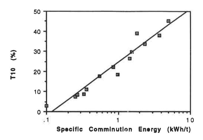
At lower energy levels the t10 - specific comminution energy relationship can be fitted using the following equation:
$$ t_{10} = a + b Ln $$ (Specific Comminution Energy) (10)
The gradient and intercept are found to vary with ore type. A breakage distribution function characteristic of a particular ore can therefore be generated from such a plot by choosing a specific energy level characteristic of the device in question.
In modelling ball mills, acceptable results have been achieved by standardising the generation of the breakage distribution function. A fixed specific breakage energy is chosen to be that obtained from an input energy of 41.788 kg-cm applied to a particle of mean size of 5.16 mm. Depending on particle sg this produces a specific energy of the order of 1-2 kWh/t. This choice of energy level was made on the basis of the fit to full scale plant data obtained by Narayanan (1985). In autogenous and semi-autogenous mill modelling the specific energy level is related to the mill diameter, the load characteristics and to particle size (Leung et al, 1987).
Since their development both the CSIRO and JKMRC ball mill models have been applied extensively and successfully in optimisation and design studies of mineral processing comminution circuits (McKee and Napier-Munn, 1990).
EXPERIMENTAL
Mill and circuit
The Hilton tower mill was a 250 kW unit from Kubota, with a grinding chamber height of 4.0 m and a diameter of 1.74 m inside liners. Make-up balls were 12.7 mm diameter.
The mill was operated in closed circuit with a cyclone. The fresh feed, a concentrate from zinc flotation, was added to the tower mill feed pump sump. The cyclone overflow passed to a low grade mineral (LGM) flotation circuit and a middling stream from LGM flotation was returned to the cyclone feed sump pump, for size separation and regrinding.
Steady state tests
Data were collected in three surveys of the tower mill circuit. Ten streams were sampled and samples were accumulated over a two-and-a-half hour period with increments taken from each stream every 15 minutes. Stream pulp densities were estimated from the wet and dry weights of the samples. The survey conditions for the tower mill itself are given in Table 1.
| Survey 1 | Survey 2 | Survey 3 | |
|---|---|---|---|
| Feed Rate (t/hr) | 16.2 | 11.6 | 7.7 |
| Feed Size (dso)(µm) | 53.6 | 52.9 | 34.9 |
| Product Size (d 50 )(µm) | 19.1 | 13.7 | 10.8 |
| Product Pulp Density (% solids) | 63.0 | 57.3 | 62.2 |
| Power Draw (kW) | 164 | 206 | 205 |
| Estimated Solids Hold-up (t) | 6.99 | 5.73 | 6.65 |
All samples were sized by wet and dry sieving down to \( 38~\mu m \) and cyclosized and decanted to produce seven - \( 38~\mu m \) size fractions. All size fractions were assayed for lead, zinc, iron, copper and sulphur.
Impulse test
The hold-up and residence time characteristics of the tower mill circuit were estimated from soluble tracer impulse tests carried out while the steady state test was in progress. A concentrated solution of lithium chloride was added to the mill feed sump at zero time and spot samples of mill discharge and cyclone underflow were collected at pre-determined time intervals over a 30 minute period. Water was decanted from each sample and assayed for lithium.
Material balances
The volumetric flow rates of the fresh feed, cyclone underflow and flotation middling streams were measured for all three surveys and were taken to be the true values. The remaining flows were estimated from size distribution splits around the cyclone and mineral phase splits around LGM flotation circuit. The consistency of the data in the tower mill circuit was very good for all three surveys (Sterns and Weller, 1992).
COMPARISON OF THE CSIRO AND JKMRC MODELS
Initially, the breakage rate parameters were calculated from the tower mill feed and discharge size distributions and mill flow rate, using both models in the way the respective groups would apply them to ball milling. Table 2 compares the experimental mill discharge size distributions with the fitted values from both models.
| Size | Mill Discha | rge - Cumulativ | e % Passing | ||||||
|---|---|---|---|---|---|---|---|---|---|
| (µm) | Survey 1 | Survey 2 | Survey 3 | ||||||
| JKMRC | EXP | CSIRO | JKMRC | EXP | CSIRO | JKMRC | EXP | CSIRO | |
| 38 | 78.7 | 78.6 | 78.0 | 85.6 | 85.3 | 85.3 | 97.9 | 97.9 | 97.9 |
| 18.8 | 48.7 | 49.4 | 49.4 | 60.8 | 62.1 | 62.2 | 73.0 | 73.1 | 73.0 |
| 9.4 | 29.5 | 28.5 | 28.5 | 37.6 | 36.0 | 36.0 | 45.1 | 45.0 | 45.0 |
| Size | Mill Discha | rge - Cumulativ | e % Passing | |||||||
|---|---|---|---|---|---|---|---|---|---|---|
| (µm) | Survey 1 | Survey 2 | Survey 3 | |||||||
| JKMRC | EXP | CSIRO | JKMRC | EXP | CSIRO | JKMRC | EXP | CSIRO | ||
| 38 | 78.6 | 78.6 | 78.0 | 85.3 | 85.3 | 85.3 | 97.9 | 97.9 | 97.9 | |
| 18.8 | 49.4 | 49.4 | 49.4 | 62.1 | 62.1 | 62.2 | 73.1 | 73.1 | 73.0 | |
| 9.4 | 28.5 | 28.5 | 28.5 | 36.0 | 36.0 | 36.0 | 45.1 | 45.0 | 45.0 | |
| Size | Mill Discharge - Cumulative % Passing | |||||||||||
|---|---|---|---|---|---|---|---|---|---|---|---|---|
| (µm) |
Increased
Feedrate |
Decreased Increased Feedrate Breakage | kage |
Decreased
Breakage |
Finer
Feed |
Coarser
Feed |
||||||
| R | ite | Ra | ate | |||||||||
| JKMRC | CSIRO | JKMRC | CSIRO | JKMRC | CSIRO | JKMRC | CSIRO | JKMRC | CSIRO | JKMRC | CSIRO | |
| 38 | 83.2 | 81.6 | 87.7 | 88.6 | 82.7 | 81.6 | 87.3 | 88.6 | 88.2 | 88.1 | 82.9 | 83.1 |
| 18.8 | 58.7 | 57.0 | 66.3 | 67.5 | 57.9 | 57.1 | 65.5 | 67.5 | 64.5 | 65.0 | 60.3 | 60.3 |
| 9.4 | 33.4 | 32.3 | 39.5 | 40.2 | 32.8 | 32.3 | 38.8 | 40.1 | 37.7 | 38.0 | 34.0 | 33.9 |
Both models fit the data well, though there was a tendency for the JKMRC model to predict more fines than that observed from the experimental data.
To test the effect of breakage distribution function choice, the Kelsall function was used in the JKMRC model, and a new fit to the data obtained. Table 3 shows that both models now give the same fit to the data. This is perhaps not surprising as the only remaining difference between the models is in the treatment of residence time distribution - three unequal mixers in series (CSIRO) compared with a single perfect mixer.
To further compare the models the parameters from one of the surveys were used to simulate the effect of changes in feed rate, feed size distribution and breakage rate. To remove the effect of the differences in choice of the breakage function, the Kelsall function was used in both models. As expected, Table 4 shows that both models return almost identical predictions.
Choice of breakage distribution function
An early finding of this exercise was that the pendulum derived ball mill breakage distribution function, when used either in the CSIRO or JKMRC ball mill models, did not provide as accurate data fits or predictions as the Kelsall function did.
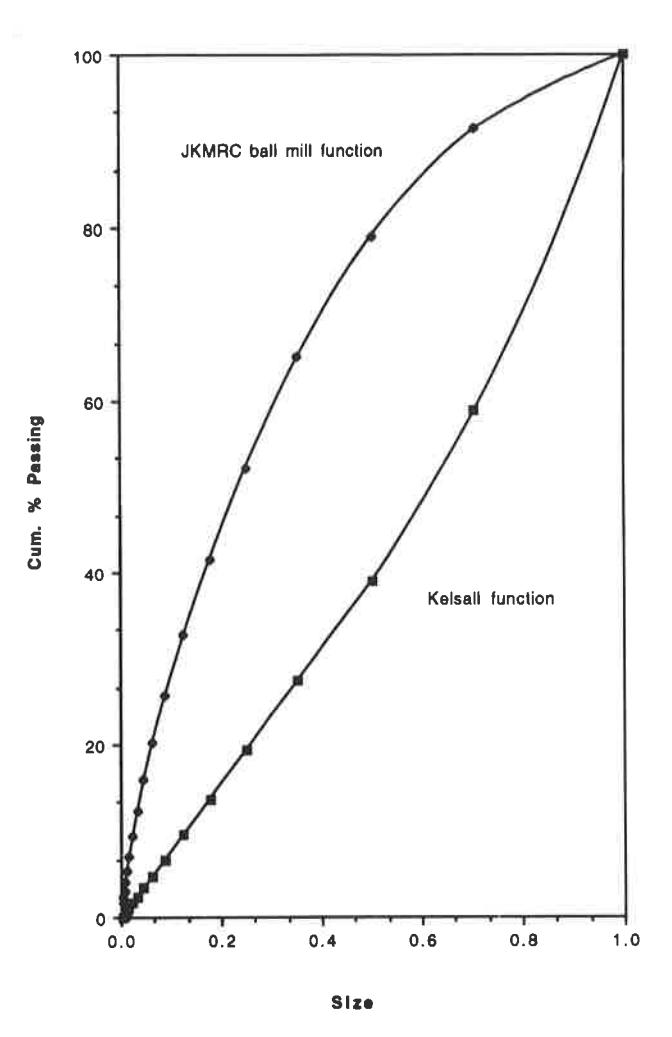
The differences between the Kelsall and JKMRC ball mill breakage distribution function is clearly seen in Figure 2. Kelsall's function which remains fixed, regardless of ore type, is much coarser than the JKMRC ball mill function.
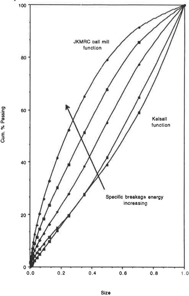
Kelsall's function can in fact be generated from pendulum test results simply by choosing a lower breakage energy. This is illustrated in Figure 3 for Hilton ore where the pendulum breakage distribution relationship with specific energy is shown.
It may be expected that the typical breakage energies developed in a tower mill are less than those in ball mills, due to the differences in charge motion between the two types of mill. By choosing a lower specific energy level to generate the breakage distribution function (one tenth that of the ball mill function) a fit to the data identical to that using the Kelsall function is obtained. This improvement over the higher energy ball mill function thus provides some evidence that lower energy breakage events may occur in tower mills. For all subsequent modelling work this lower energy breakage function has been used in the JKMRC model as being characteristic of breakage in tower mills.
VALIDATION OF THE MODELS
The operating conditions of the three surveys for which data were obtained varied considerably in terms of feed rate, power draw (ball charge) and feed size distributions. Table 1 summarises these conditions. To validate the models' predictive capability it was therefore decided to take the parameters fitted to the data from survey 2 and use them to simulate the tower mill performance under the conditions of surveys 1 and 3.
The data show very similar trends from the CSIRO and JKMRC models when the latter uses a lower energy breakage distribution function. Both models predict the observed data very well.
PREDICTING FULL SCALE TOWER MILL PLANT PERFORMANCE USING PILOT MILL DATA
In conjunction with surveys of the Hilton full scale tower mill, testwork was also undertaken on a pilot scale tower mill treating Hilton ore. The 1.5 kw pilot mill was run in closed circuit with a sump and pump under a variety of ball charge, ball size and feed slurry conditions. While running, samples were taken at timed intervals and subsequently sized. By using results from consecutive timed samples, the mill was modelled by assuming it was running under pseudo-continuous operation.
It was considered that the principal factors which determine the rate of breakage in a tower mill are the number of balls and the velocity which is imparted to them. These two factors are related to the following variables:
- stirrer diameter (Ds)
- height of ball charge (H)
- pitch (P)
- number of starts (S)
- mean ball diameter (DB)
- stirrer rpm (N)
The number of balls which are moved is related to the stirrer diameter, ball charge height and ball size:
Number balls $$ \quad \alpha \quad \frac{D_s^{\ 2}H}{D_B^{\ 3}} $$
As attrition is believed to be the principal mode of breakage in a tower mill then the rate of breakage would be expected to be related to the ball surface area:
Ball surface area $$ \alpha = \frac{D_s^2 H}{D_B} $$
The rate at which balls are moved is related to the stirrer diameter, speed of the stirrer and the number of turns that it has per unit height which are immersed in the ball bed:
Rate at which balls moved $$ \alpha = \frac{D_S N S}{P} $$
Multiplying the ball surface area and ball movement rate terms together thus provides the following dependence of the specific rate of breakage:
Specific Rate of Breakage $$ \alpha = \frac{D_s^3 \text{ HNS}}{D_B P} $$
The pilot mill breakage rates were scaled using this relationship and used to predict the tower mill discharge size distribution from the full scale tower mill. The results are shown in Table 6. The results show good agreement with experimental data. It is too early, however, to confirm the general accuracy of this technique. To do so, further data, which are being collected, is required:
| Size | Mill Discharge - Cumulative % Passing | ||||||||||
|---|---|---|---|---|---|---|---|---|---|---|---|
| (μm) | Sur | vey 1 | Survey 3 | ||||||||
|
CSIRO
(Kelsall) |
EXP |
JKMRC
(tower mill) |
JKMRC
(ball) |
CSIRO
(kelsall) |
EXP | JKMRC (tower mill) |
JKMRC
(ball) |
||||
| 38 | 75.6 | 78.6 | 77.2 | 77.7 | 93.8 | 97.9 | 93.8 | 93.7 | |||
| 18.8 | 49.3 | 49.4 | 50.0 | 51.8 | 73.5 | 73.1 | 74.4 | 65.4 | |||
| 9.4 | 27.4 | 28.5 | 27.8 | 31.9 | 43.7 | 45.0 | 45,7 | 39.8 | |||
| Size | Mill Discharge - Cumulation % Passing | |||||||||
|---|---|---|---|---|---|---|---|---|---|---|
| (µm) | Su | rvey 1 | Sur | vey 2 | Survey 3 | |||||
| Ехр | Predicted | Ехр | Predicted | Ехр | Predicted | |||||
| 38 | 78.6 | 75.6 | 85.3 | 84.0 | 97.9 | 93.2 | ||||
| 18.8 | 49.4 | 47.8 | 62.1 | 59.7 | 73.1 | 72.2 | ||||
| 9.4 | 28.5 | 26.4 | 36.0 | 34.2 | 45.0 | 43.5 | ||||
CONCLUSIONS
From analysis of the Hilton tower mill data it has been found that little difference exists between the contents based models of the JKMRC and the population balance models of the CSIRO, apart from their choice of breakage distribution function. The CSIRO uses a fixed function proposed by Kelsall which was found to enable good data fitting and predictive capability. The JKMRC model uses an ore specific breakage distribution function obtained from breakage of the relevant ore in a twin pendulum device. Similar performance to the CSIRO model was found when using the JKMRC model, providing a lower energy breakage distribution function than used for ball milling was utilised. It can be inferred from this latter result that breakage within a tower mill takes place at energy levels much lower than found in ball mills.
As tower mills undoubtedly utilise attrition as the predominant mode of breakage, the use of an impact device such as a pendulum may not be the most appropriate for determining the breakage distribution function. Investigations are currently underway into alternative methods for determining this function which better reflect the operation of tower and stirred mills.
The success of the JKMRC and CSIRO models in describing the Hilton tower mill performance, both from full scale and pilot scale mill data, will ensure their further use in this field. They are limited, however, in terms of their ability to simulate the effects of design changes, and rely heavily on empirical relationships for their use to predict anything other than relatively simple changes to operating conditions. Whilst such models will continue to be used for optimisation and scale up, it is believed that a more fundamental approach is required. To this end studies are underway using a transparent laboratory model to provide information on the motion of the media and slurry charges. This information will be incorporated in a mechanistic stirred mill mathematical model whose structure is currently under development.
ACKNOWLEDGEMENTS
The authors would like to thank Mount Isa Mines for permission to use the data from their Hilton Concentrator in this paper and for the assistance of their staff in collecting the data. The sponsors of the AMIRA P336 Fine Grinding project who sponsored this research are also gratefully acknowledged. The authors also thank Mr M Duffy of the JKMRC for collecting the pilot tower mill data and Dr T J Napier-Munn for his useful suggestions on the structure and content of the paper.
REFERENCES
- Austin L G, 1971. A review introduction to the mathematical description of grinding as a rate process. Powder Technol , 5:(1)1-17.
- Heyes G W, Kelsall D F and Stewart P S B, 1973b. Continuous grinding in a small wet rod mill. Part II. Breakage of some common ore minerals. Powder Technol , 7:(6)337-341.
- Kavetsky A and Whiten W J, 1982. Scale-up relations for industrial ball mills. Proc Australas Inst Min Metall, 282:47-55.
- Kelsall D F, Reid K J and Stewart P S B, 1969. The study of grinding processes by dynamic modelling. Electr Eng Trans Inst Eng , Aust, EE5(1):155-169.
- Leung K, Morrison R D and Whiten W J, 1987. An energy based ore specific model for autogenous and semi-autogenous grinding. Copper 87, Santiago, Chile.
- McKee D J and Napier-Munn T J, 1990. The status of comminution simulation in Australia, Minerals Engineering, 3:(1/2)7-21.
- Narayanan S S and Whiten W J, 1983. Breakage characteristics of ores for ball mill modelling, Proc Australas Inst Min and Metall, 286, June, pp 31-39.
- Reid K J and Stewart P S B, 1970. An analogue model of batch grinding and its application to the analysis of grinding results. Chemeca 70, pp 87-106.
- Sterns U J and Weller K R, 1992. Assessment of the low grade mineral circuit surveys at Hilton 1991. CSIRO Div Mineral and Process Engineering. Limited circulation. Report REP 709.
- Weller K R, 1981. Hold-up and residence time characteristics of full scale grinding circuits. (Eds: J O'Shea and M Polis), Automation in Mining, Mineral and Metal Processing (IFAC). Pergamon, Oxford, pp 303-307.
- Whiten W J, 1974. A matrix theory of comminution machines, Chemical Engineering Science , 29:(588-599)31-39.