THE DEVELOPMENT OF A DYNAMIC MODEL FOR AUTOGENOUS AND SEMI-AUTOGENOUS GRINDING

W. VALERY Jnr and S. MORRELL

Julius Kruttschnitt Mineral Research Centre, University of Queensland, Isles Road, lndooroopilly, Qld 4068, Australia

ABSTRACT

To assist in the study and understanding of plant dynamics, circuit interactions, mill operational behaviour and automatic control schemes, a model of the dynamic behaviour of autogenous (ag) and semi-autogenous mills (sag) is currently under development at the JKMRC. The model is being developed to provide an accurate dynamic response in terms of power draw, grinding charge level, slurry level and product size distribution for changes in feedrate, feed size, feed hardness and water addition. The conceptual structure of the model is described together with dynamic data from 2 full scale high aspect ratio autogenous mills which will be used to validate the model. The data were obtained from a series of step tests and comprise trends in power draw, bearing pressure, solids and waterfiowrates as well as an indication of the fraction of coarse rocks in the feed. This latter quantity was obtained from a novel, yet simple device for counting rocks which will · be described. The mills measured response to these step changes is presented together with an explanation for their behaviour in terms of the physical changes which took place inside the mill.

Keywords

,Grinding, autogenous, semi-autogenous, mill, dynamic model, simulation

INTRODUCTION

For effective AG/SAG mill operation and control, the measurement and control of important mill variables such as feed size, ore hardness and mill load are desired, but not always possible. The lack of available instrumentation to measure these variables is one factor which has impeded the development of more advanced and effective AG/SAG mill control. One solution to such a problem is a dynamic model that can be used to predict information about the process that cannot be easily measured.

In this paper a conceptual model is described which is being developed to provide accurate dynamic response in terms of power draw, rock and slurry levels as well as product size distribution. Dynamic data which have been collected to assist with the development and validation of the model are presented together with an interpretation of the observed trends and the way in which the proposed model will reproduce them.

DYNAMIC MODEL STRUCTURE

The model chosen to provide the dynamic structure is Whiten's contents based model [1]. The model comprises two equations which can be written as:

$$ \frac{dS_{i}(t)}{dt} = f_{i} - p_{i} + \sum_{j=1}^{i-1} a_{ij} \cdot r_{j} \cdot s_{i} - (r_{i} \cdot s_{i} - a_{ii} \cdot r_{i} \cdot s_{i}) $$ (1)

where:

\( s_i(t) \) : is the mass of material in size class i, at time t, within the mill, fi. is the total flow rate of feed material in this size class,

p_i: is the total flow rate of discharge material in this class,

r_i: is the rate at which particles in size class i break, a_ii: is the breakage distribution or appearance function which describes the fraction of material breaking into size class i due to breakage of size class j, and discharge rate of class size i.

The solution to equations 1 and 2 provides predictions of the product size distribution, load size distribution and load mass and is found via the use of a computer based algorithm which is outlined in schematic form in Figure 1.

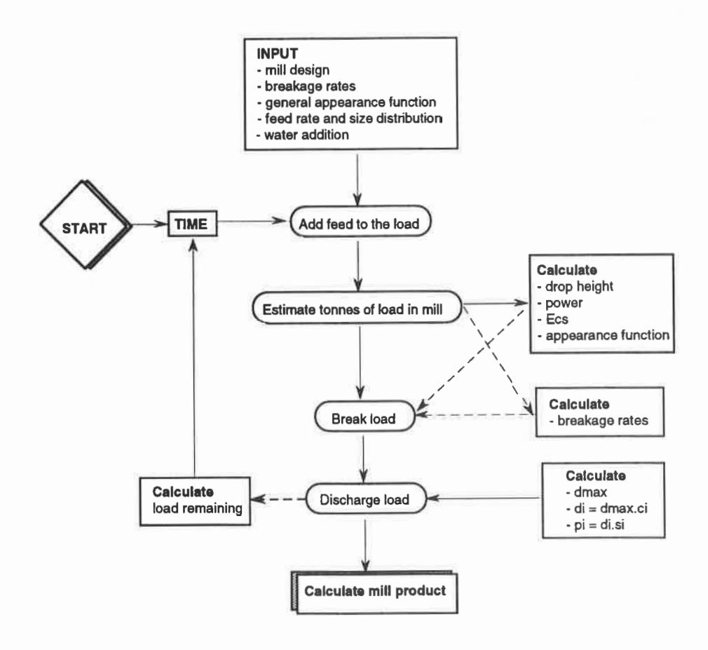
The programs being developed for the dynamic simulation model are compatible with the existing steady state simulation models available at the JKMRC. Subroutines are used to simulate the physical processes involved and a time-sequencing subroutine is proposed which controls the operation of events within the program, including the integration step.

The model contains 3 parameters which must be determined before the equations 1 and 2 can be solved. These are:

• the breakage rates (r_i) which can be regarded as the breakage frequency and which vary with factors such as mill speed and charge size distribution [2]
• the appearance function \( (a_{ij}) \) which describes the size distribution of the products from breakage events and which is a function of the ore type and the specific breakage energy.
• the discharge rate (di) which relates the load to the flowrate of products out of the mill. It is a lumped parameter which contains both the effect of classification of solids by the grate and fluid flow effects which are related to the hold-up of slurry in the mill.

Breakage Rate Function

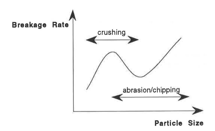
The breakage rate is related to particle size and typically takes the form shown in Figure 2. The breakage rate function shape is largely governed by the mill load particle size distribution and mill speed. In this model the breakage rates are related to the load size distribution via empirical equations determined from a large number of pilot and full scale mills where the load size distributions were measured. Fine tuning of the equations will be necessary for a particular mill using results from steady-state testwork.

Appearance Function

The appearance or breakage distribution function describes the size distribution from a breakage event. It is dependent upon both the ore type and the specific energy associated with the breakage event. The model relies on the use of laboratory tumbling and impact breakage tests of the relevant ore to provide a relationship between the specific energy and the appearance function. The results are conveniently represented in a relationship between the specific energy and the breakage product parameter \( t_{10} \) as follows:

$$ t_{10} = A [1 - e^{(-b. Ecs)}] $$ (3)

where

A, b: are the ore specific constants, and Ecs: is the specific comminution energy (kWh/t).

It has been shown [1] that the \( t_{10} \) , which is defined as the fraction of broken product which is smaller than one tenth of the original particle size, can be easily related to the entire product size distribution. Equation 3 can therefore be used to generate the entire product size distribution for a given specific energy. A more detailed description of the data treatment process can be found elsewhere [1].

Whilst the laboratory tests provide a relationship between specific energy and size reduction, the specific energy of breakage events within the mill must still be estimated. This will vary with such factors as mill diameter, speed, charge density and charge level. Within the model a simplified description of the charge shape and motion is used to calculate the mean height to which the charge is raised, dropped and subsequently broken [2,3]. This is then related to the specific energy of breakage for each particle size.

Discharge and Classification Functions

The discharge rate (d_i) is considered to be the product of two mechanisms:

• fluid transport through the grate, and
• solids classification by the grate.

Within the model, \( d_i \) is related to the contents and product using equation 2. This equation can be expanded to incorporate a dimensionless classification parameter \( (c_i) \) and a fluid flow-related parameter \( (d_{max}) \) :

$$ p_i = s_i (d_{max} \cdot c_i) $$ (4)

The classification parameter (c_i) is related to the grate aperture of the mill as shown in Figure 3 [4].

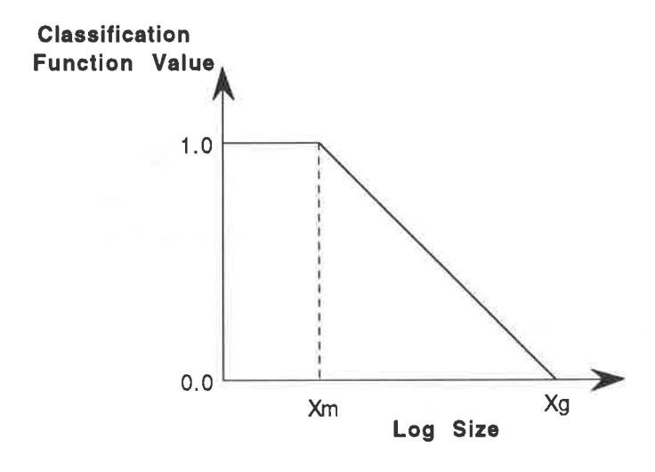
The value of Xg is the effective grate aperture, whilst Xm is the maximum particle size which behaves "like water", ie. is not subject to classification. The function allows for no classification of particles above the grate size (Xg) but varying degrees of classification for particles below the grate size but above Xm.

Whereas the classification parameter relates to solids behaviour, the \( d_{max} \) parameter relates to the proportion of the slurry which acts like a fluid. By definition this material has a classification function value of unity. Hence from equation 4 \( d_{max} \) can be defined as:

where

\( \Sigma p_i \) = flowrate of slurry out of the mill \( \Sigma s_i \) = hold-up of slurry in the mill

To determine what the value of d_max is therefore requires a relationship between slurry hold-up and slurry flowrate out of the mill. It has been found [5] that the relationship between flowrate and hold-up can be expressed using 2 equations, depending upon whether flow occurs via the grinding media or via a slurry pool which may form at the toe of charge at higher flowrates (Figure 4).

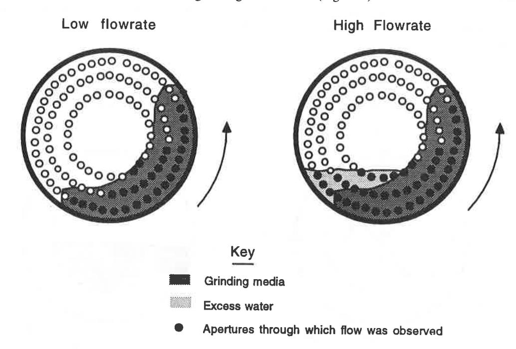
The equations are as follows:

Flow via the grinding media:

$$ Q_{\rm m} = k_{\rm m} \cdot J_{\rm pm} \cdot \gamma^{2.5} \cdot D^{0.5} \cdot A \cdot \emptyset^{-1.38} $$ (6)

Flow via the slurry pool:

$$ Q_t = k_t \cdot J_{pt} \cdot \gamma^2 \cdot D^{0.5} \cdot A $$ (7)

where

\( Q_t \) : is the volumetric discharge flowrate through the grinding media(m³/hr), \( Q_m \) : is the volumetric discharge flowrate through the slurry pool(m³/hr), is the fractional slurry hold up in the grinding media

J_pt: is the fractional slurry hold up in the slurry pool γ: grate design parameter D: is the mill diameter (m), A: is the total open area of grate apertures (m²), ø: is the fraction of critical speed, and \( k_t \) , \( k_m \) are constants.

Apart from being used to estimate \( d_{max} \) , equations 6 and 7 are used to determine whether flow is occurring only via the grinding media or whether a slurry pool has also formed. In the case of the latter the slurry pool level may also be determined and its effect on power draw estimated using the JKMRC's power model [3].

Power Draw

Solution of the grinding model equations 1 and 2 gives predictions of the product size distribution, charge size distribution and charge mass. Given the charge mass, mill dimensions and mill speed, the power draw can also be estimated. For this purpose the JKMRC's power model is used [6]. This model utilises the same simplified charge shape and motion that provide the drop height data for the appearance function calculations (Figure 5).

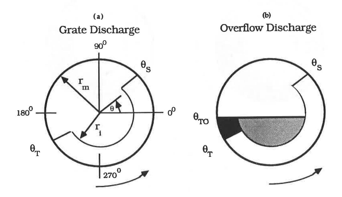
The power model equation has the following form:

$$ Power\alpha \int_{0}^{m} \left\{ VrLrg[\rho c(\sin\theta s - \sin\theta T) + \rho p(\sin\theta T - \sin\theta TO)] + 0.5Vr^{3}L\rho x \right\} $$ (8)

where

L: length of cylindrical section of the mill liners (m)

r: radial position (m)

r_i: radial position of the charge inner surface (m)

r_m: radius of the mill inside liners (m)

V_r: tangential velocity of a particle at radial distance r (m.sec^-1)

\( \begin{array}{ll} \theta_s \colon & \text{angular displacement of shoulder position at the mill shell (rads)} \\ \theta_T \colon & \text{angular displacement of toe position at the mill shell (rads)} \\ \theta_{TO} \colon & \text{angular displacement of surface of slurry pool at the toe (rads)} \\ \rho_c \colon & \text{density of total charge (excluding excess slurry) (t.m}^{-3}) \end{array} \)

\( \rho_p \) : density of the excess slurry (t.m^-3)

In cases where slurry flow is only through the grinding media the charge pattern shown in Figure 5 (a) will apply, in which case there will be no slurry pool and \( \theta_{TO} \) will equal \( \theta_{T} \) . The second term in equation 8 will therefore equal zero. Where, using equations 6 and 7, a slurry pool is indicated to have formed, \( \theta_{TO} \) can be calculated. From equation 8 it can be seen that in this case the second term will be negative giving rise to a lower power draw. In this way the model should be able to mimic the power and load trends associated with changes in flowrate to the mill, including the effect of the formation of a slurry pool.

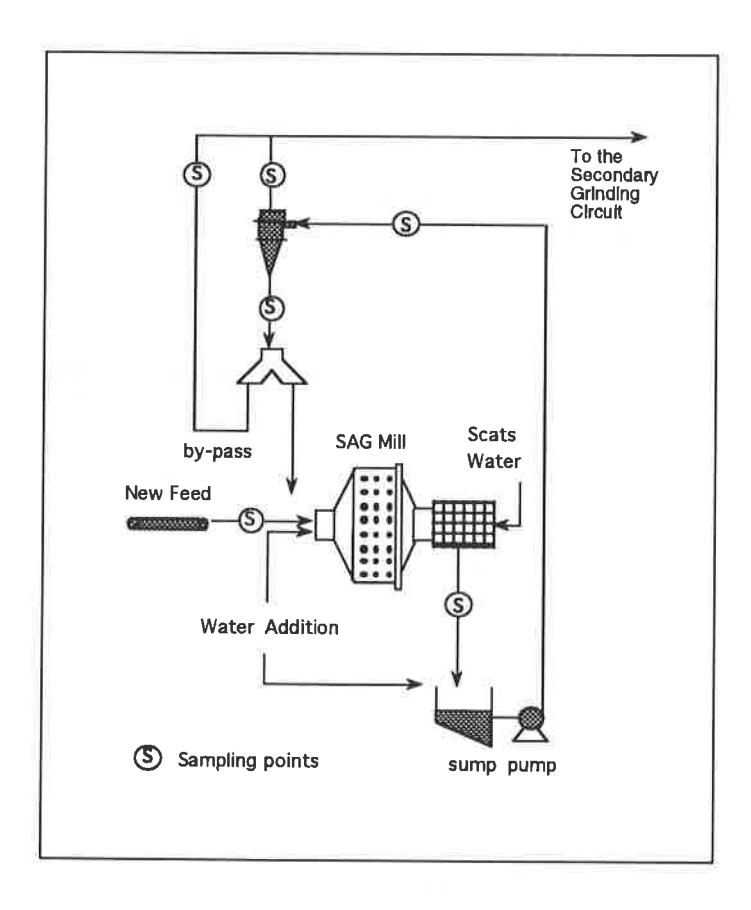
In practice the effect of a slurry pool is to reduce the power draw. This can manifest itself in closed circuit mills as an observed association between the amount of recycle and the power draw, which drops as the recycle increases [7]. The magnitude of the effect varies and in extreme cases can cause considerable power reduction [8]. The effect is illustrated using data recorded from Mount Isa Mine's copper concentrator ag mill. In this experiment the mill was configured such that its discharge was pumped to a cyclone, the underflow from which could be either diverted back to the mill or combined with the cyclone overflow and sent to the ball mill (Figure 6). In this way the recycle load could be accurately controlled.

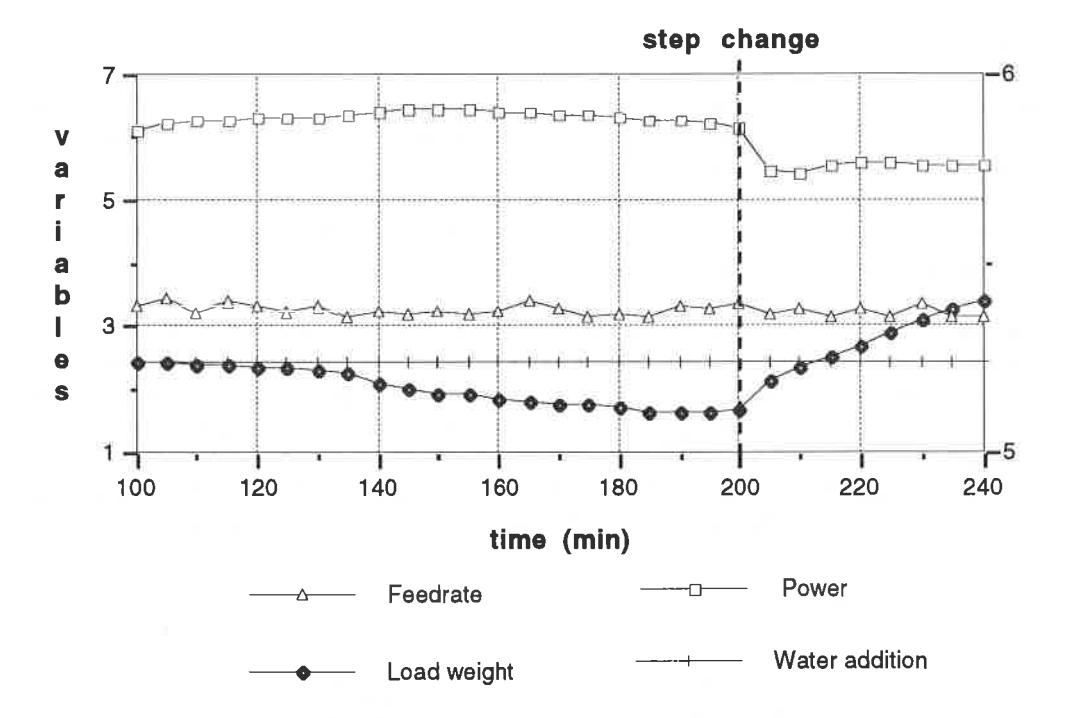
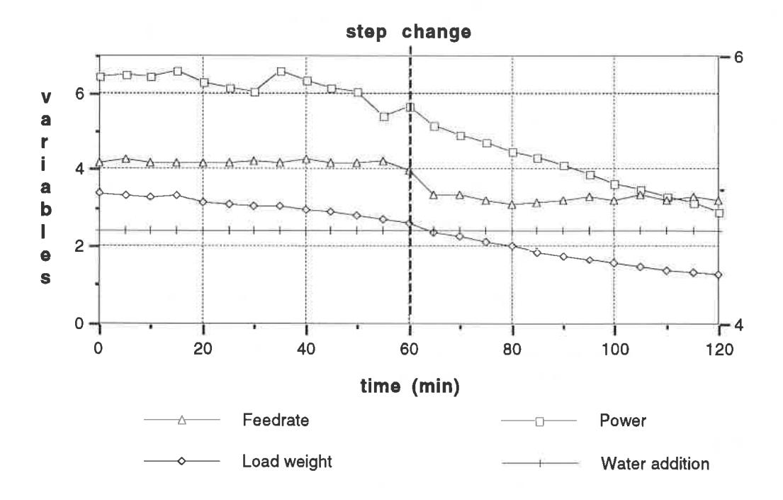
Initially the mill was run in open circuit with all the cyclone underflow being diverted with the overflow to the ball mill. At time equals to 200 minutes 70% of the cyclone underflow was returned to the ag mill feed. From Figure 7 it can be seen that the bearing pressure increases in response to the accumulation of slurry in the slurry pool, whilst at the same time the power drops and remains at the lower level. This effect of increasing load yet decreasing power should not be confused with that associated with a mill which has an excessive grinding media charge ie greater than 45–50% of mill volume. Although the symptoms may be similar the causes are different.

Further confirmation of the effect of the slurry pool can be seen in Figure 8 where the feed was subsequently stopped to the mill (time = 175 min). Contrary to normal open circuit conditions where

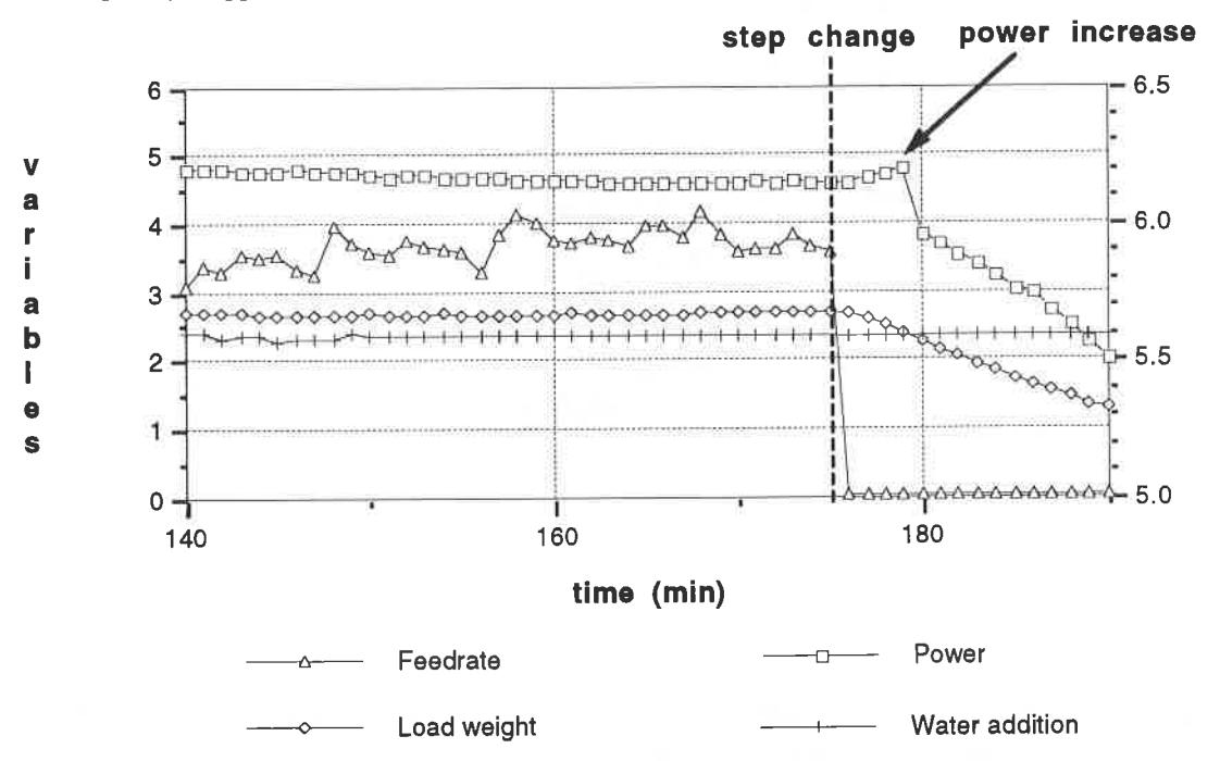
the power would normally drop in response to a reduction in feedrate (Figure 9), in this case the power initially climbs as the slurry in the pool flows out of the mill. This effect takes a relatively short time to occur (the variables are plotted for each minute instead of an average of 5 minutes in the other figures) due to the fast slurry drainage. The reduction in the load mass due to grinding out then exerts an influence and the power then drops in a predicted manner.

Effect of Water Addition

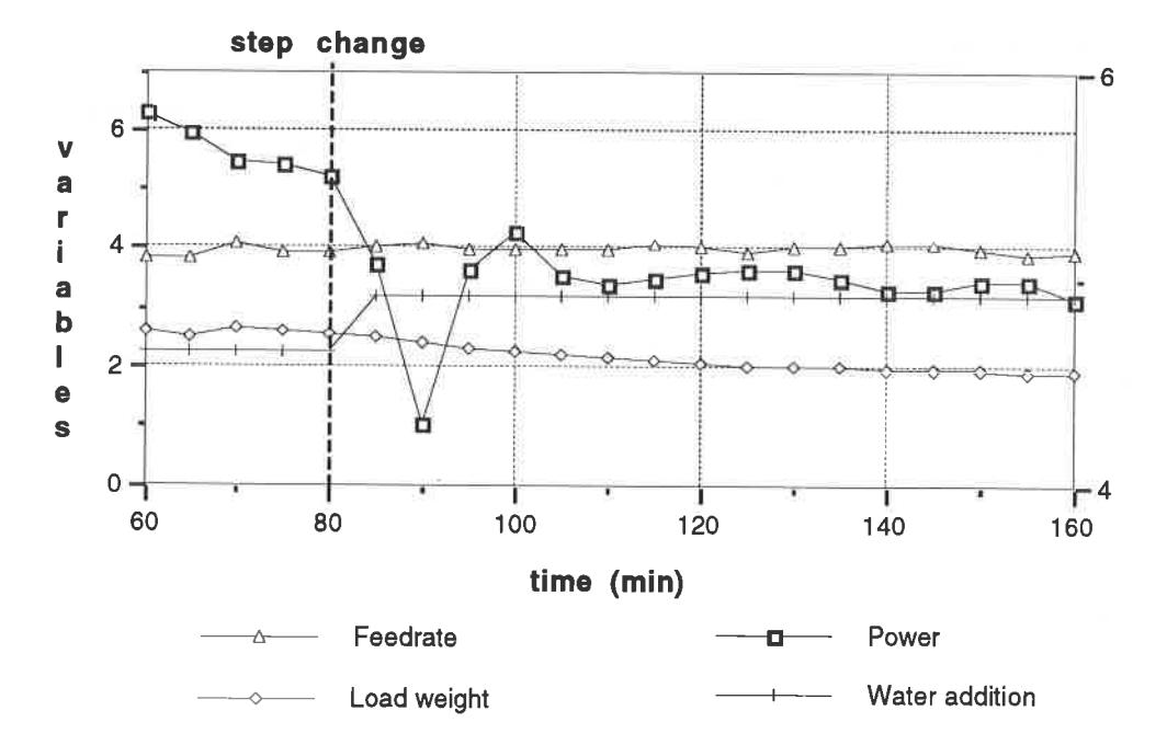
Rapidly increasing water addition to a mill is often used by operators to quickly reduce the power draw when it threatens to exceed overload levels. Once again using data from the MIM copper concentrator ag mill the effect is illustrated well (Figure 10). It can be seen at time = 80 minutes the water addition to the mill was increased from 223 m3/hr to 316 m3/hr. Although the power draw can be seen to have been slowly declining the addition of the extra water causes a very sharp drop in the power draw. Unlike the previous case where an increase in slurry to the mill caused a lasting drop in power, when the water was increased the power drop was temporary and began to climb back up after 10 minutes. In this case the initial effect of the water surge is to flush accumulated finer solids out of the mill and hence the charge density and power draw decreased. It is possible that if the water increase is large enough a slurry pool may also form and further assist with the drop in power. However as the finer solids are flushed out the grinding media voidage will increase, allowing the slurry level to drop. Fine solids will then begin to accumulate, causing the power draw to rise again. Interestingly, the charge mass, as indicated by the bearing pressure (load weight in the Figure 10), did not drop when the water was increased. This may be due to some compensation associated with build-up of water and a simultaneous loss in fines. In other mills studied it has been found that charge mass initially decreases as the water is increased.

Within the model the increase in water flowrate will be reflected in an initial increase in dmax and hence a corresponding increase flow of solids out of the mill. The power will also be predicted to drop due to the decrease in charge density. Following the loss of fine solids the slurry level will drop causing dmax to decrease and the fine solids, charge density and power draw to increase again.

Feed Size Effects

Feed size distribution changes are one of the most common causes of erratic behaviour in ag and sag mills. This results from the grinding media being obtained from the feed. From this, it naturally follows that the behaviour of the mill will also be dependent on the feed size distribution. In the model, as the feed size distribution varies the load size distribution will also vary. The breakage rate distribution will then change and in turn cause a change in the load size distribution. This process will iterate until steady state is predicted to have been reached.

Measurement of the dynamic response to changes in the feed size distribution are difficult to obtain, making the task of validation of the models response equally difficult. This is due to the problems of measuring feed size distributions on-line. In an attempt to obtain on-line size data a simple rock counter was developed and installed at 2 sites. An infrared sensor was installed on the feed belt with the beam being transmitted and reflected across the belt. The sensor was placed at the feed chute (the flattest part of the belt) to avoid counting rock piles. The aim of this instrument was to measure the number of rocks per minute larger than a certain size as defined by the height of the beam (i.e. larger than 200 mm at Mount Isa and larger than 100 mm at Hellyer). Each time the infra red beam was interrupted by coarse rocks, a digital signal was sent to the control system. The output of this "rock counter" was monitored and recorded as the number of rocks per minute larger than a certain size. It was found, however, that although some significant trends were sometimes apparent, for much of the time little association between the frequency of coarse rocks and mill behaviour was seen. This is due to the fact that the feed size distribution is just, if not more, important than the amount of coarse rocks.

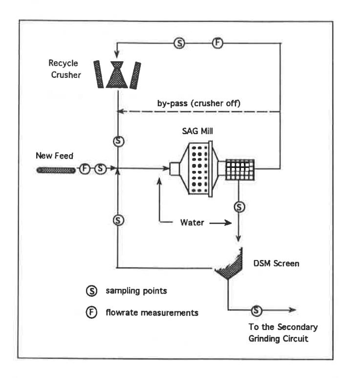
This latter fact is clearly shown from testwork conducted at the Hellyer Mine. The circuit is shown in Figure 11. The mill is a high aspect ratio ag mill in closed circuit with a pebble crusher and DSM screens.

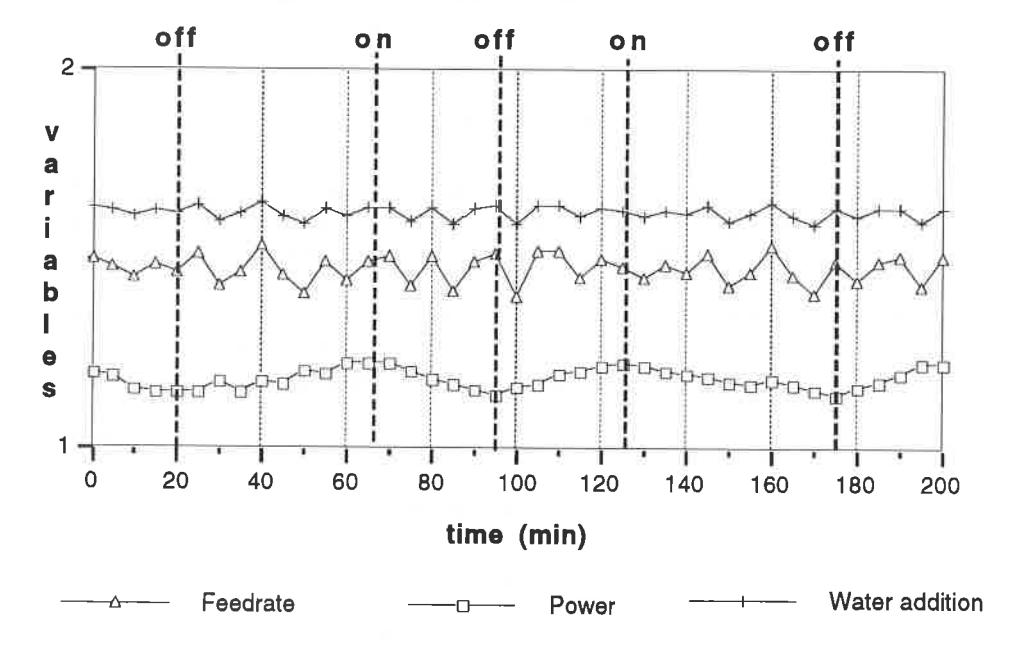
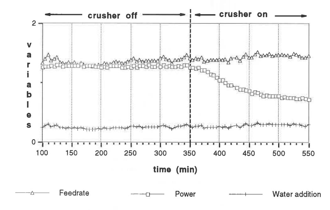
The pebble crusher circuit is configured such that the crusher can be easily by-passed, in which case the pebble stream is returned to the mill. The mine uses this facility in a novel manner to tightly control the mill power in a very narrow band. This is done by an automatic control scheme which brings the crusher on line when the power draw reaches an upper limit and takes the crusher off line when the power drops below a lower limit. The action of this control strategy is clearly illustrated in Figure 12. When the crusher is brought on line the power immediately begins to drop. Although there is no load indication for this mill it is most likely that the load level would also be falling. When the crusher goes off line the power (and load level) begin to rise again. This produces the oscillating power trend seen in Figure 12. It is pointed out that the amplitude of the oscillations is approximately 20 kW with a mean power draw of 1440 kW.

In terms of the feed size distribution to the mill, the effect of the recycle crusher is to substantially modify it. The action of the recycle crusher can therefore be viewed as causing a step change in the feed size distribution. The reason for the observed effect of the crusher has to do with the influence of the so-called critical size fraction in the mill. This is typically in the 25–50mm size range. In many mills it will be found that this fraction constitutes a very large proportion of the mill load. It is therefore responsible for drawing a significant amount of power as well as occupying a large amount of mill volume. By extracting a large proportion of this material and reducing it to a size which can exit the circuit and/or is better able to be ground by the mill, reductions in mill load and power can be achieved. The effect is much more noticeable when the crusher is kept on line as can be seen in Figure 13. Mill power in this case falls by 35% yet the throughput increases by 15%.

CONCLUSIONS

A conceptual dynamic ag/sag mill model has been developed for the prediction of the power draw, load level and product size distribution. The structure of the model is such that it should provide realistic responses to changes in feedrate, water addition, recycle load, feed size distribution and ore hardness.

Dynamic data have been collected from a number of mills to assist with the development and validation of the model. Further data will be collected on the speed response of mills to enhance this data base. The projected outcome from the project will be a versatile dynamic model proven using a wide range of industrial data.

ACKNOWLEDGMENTS

The authors thank the financial support from CNPq (Brazil) through the "Young Scientist Award Scholarship" as well as the "JKMRC Post Graduate Student Award". The contributions of Mount Isa Mines and Hellyer (Aberfoyle Resources Ltd.) through the Australian Mineral Industries Research Association (AMIRA Project P9) are also gratefully acknowledged. The authors would also like to thank Don McKee, Toni Kojovic and Adrian Dance for their kind cooperation in this study.

REFERENCES

• 1. Whiten, W.J., A matrix theory of comminution machines, Chem. Eng. Sci. No. 29:585-599, (1974).
• 2. Morrell, S., et al., Power Draw of Grinding Mills Its measurements and Prediction, Proc. Fifth Mill Operators Conference, Roxby Downs, Australia, AusIMM, 109–114 (1994).
• 3. Morrell, S., et al., The Prediction of Power Draw in Wet Tumbling Mills, Ph.D. Thesis, The University of Queensland, Australia, (1993).
• 4. Leung, K., An Energy Based Ore Specific Model for Autogenous and Semi-Autogenous Grinding Mills, PhD Thesis , The University of Queensland, Australia, (1987).
• 5. Morrell, S. & Stephenson, I., Slurry Discharge Capacity of Autogenous and Semi-Autogenous Mills and the Effect of Grate Design, Int. Journal of Minerals Processing , Elsevier, In Press, (1995).
• 6. Morrell, S., The Prediction of Grinding Mill Power, Trans IMM , 101, C25-32, (1991).
• 7. Morrell, S., Simulations of Bauxite Grinding in a Semi-Autogenous Mill and DSM Screen Circuit, M.Eng.Sc Thesis , The University of Queensland, Australia, (1989).
• 8. Warder, J. & Davies, M., Autogenous milling at Leinster Nickel Operations, Proc. Fifth Mill Ops. Conf. , Roxby Downs, AusIMM 115–121 (1994).