



The content on this page was automatically generated from the PDF publication document and may contain errors or inaccuracies. Please refer to the original PDF for the most accurate information.
THE INFLUENCE OF SLURRY TRANSPORT ON THE POWER DRAW OF AUTOGENOUS AND SEMI-AUTOGENOUS MILLS
Dr. S. Morrell' and Dr. T. Kojovic2 1- Manager - Comminution Research, 2- Senior Research Fellow Julius Kruttschnitt Mineral Research Centre Isles Road, Indooroopilly, Brisbane, Australia
ABSTRACT
In recent years there has been a trend in Australia towards closecircuiting autogenous and semi-autogenous mills with hydrocyclones. This has resulted in attention being focussed on issues relating to the ability of the grates and pulp lifters to effeciently remove slurry from the mill. This paper describes the deleterious effects on power draw and mill performance that have been observed to occur due to poor slurry transport. Mechanisms which explain these phenomena are described. These are used to develop mathematical models which link grate flow capacity to slurry hold-up and power draw. The model's ability to predict flow capacity and its effect on power draw is illustrated using industrial data.
INTRODUCTION
Recent experience with a number of autogenous (ag) and semiautogenous (sag) mills in Australia has highlighted the importance of efficient slurry transport related to power draw and throughput.
This has come about following initial problems that were experienced at WMC's Leinster and MIM's copper concentrator circuits where their large diameter autogenous mills were run in closed circuit with cyclones (Warder and Davies, 1994; Leung, Lumsdaine and Veran, 1992). In these cases atypically low power draws and lower than expected new feedrates were experienced. These symptoms were believed to be associated with the closed circuit operation of both mills. The association between closed circuiting (more specifically recycle load) and a drop in power draw is not new (Morrell, 1989). From analysis of power draw and recycle load data from Alcoa's Pinjarra sag mill, which is in closed circuit with DSM screens, the following empirical relationship was obtained:
Power (kW) = 495 + (1 2.19*charge mass) - (693.1 *recycle fraction)
where recycle fraction is the recycle tonnage rate divided by the total feedrate to the mill and charge mass is measured in tonnes. However, it is not the recycle load per se which influences the power but the total volumetric flowrate of slurry, which is relatively high in closed circuits, and the resultant hold-up both of which increase as the recycle load increases. This results in an increase in the mass of the mill contents yet the power draw drops - contrary to the expected trends in cases other than where the volumetric load has exceeded about 45-50% of mill volume (Morrell, 1996).
In this paper the relationship between volumetric flowrate of slurry, hold-up and power draw will be illustrated and discussed with particular reference to the data collected from the a large diameter mill.
SLURRY FLOW IN GRATE DISCHARGE MILLS
With one or two exceptions (Gupta et a1,1981; Moys, 1986) in the past the study of flow through grate discharge mills has been severely limited. More recently a programme of research at the JKMRC has been instigated in which the relationship between hold-up and flowrate and the influence of mill speed and grate design have been studied as well as the role of the pulp lifters. From the initial results of this work (Morrell and Stephenson, 1996) flow was found to take place in two distinct zones depending on the magnitude of the flowrate (Figure 1).
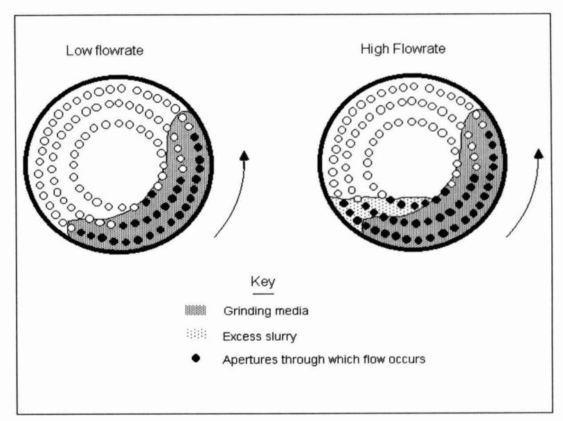
The zones are those associated with the grinding media and at the toe of the charge where a slurry pool forms once the interstices of the grinding media are fully occupied. Hence at lower flowrates flow is seen to occur only via the grinding charge and subsequently via the grate apertures which come into contact with the part of the charge which contains the slurry hold-up. As the flowrate is increased the slurry hold-up increases and more and more of the grinding charge interstices are occcupied by the slurry. Hence more of the grate apertures are in contact with the hold-up resulting in increased flow out of the mill. Eventually, however, all of the grinding charge interstices become occupied with slurry. Further increases in flow result in the hold-up accumulating in the toe region where flow via the grate apertures also occurs. Flow via the two zones has been found to be related to the hold-up, mill speed etc. in a different manner. This gives rise to two different equations for the flowrate - hold-up relationship. These are as follows (Morrell and Stephenson, 1996):
$$ J_{pm} = k_m Q_m^{0.5} \gamma^{-1.25} A^{-0.5} \phi^{0.67} D^{-0.25} ; J_p < J_{max} $$ $$ ; J_{pm} = J_p $$ (1)
$$ J_{pt} = \kappa_t Q_t \gamma^{-2} A^{-1} D^{-0.5} $$ ; \( J_p > J_{ma} \) ; \( J_{pt} = J_p - J_{max} \) (2)
where
Jpm = fraction of mill volume occupied by slurry in the grinding media zone
Jpt = fraction of mill volume occupied by slurry in the toe zone
Jp = fraction of mill volume occupied by slurry
J, = fraction of mill volume occupied by grinding media plus associated interstices
J, = "dead" slurry hold-up fractio = 0.33 (1-r,) (4)
r, = relative radial position of the outermost row of grates
Q,; Q, = volumetric flowrates via the grinding media and toe zones respectively
Y = grate design parameter related to position of apertures
a, = open area of grate apertures at radial position r,
r, = radius of mill inside liners
A = grate open area
4 = fraction of critical speed
D = mill diameter
k,; k, = calibration constants which are approximately equal to 0.013 and 0.001 repectively
Of particular importance in equations (1) and (2) is J,,,, which is the hold-up beyond which slurry begins to accumulate in the toe region, and its relationship to J, which is the fraction of the rnill occupied by grinding media. The significance of this relationship is that the volume of grinding media affects slurry flow and in particular controls at what point slurry will begin to accumulate in the toe region. With low grinding media volumes, slurry will begin to accumulate in the toe region at much lower flowrates than with higher volumes. This factor is particularly important with autogenous mills in which the grinding media derive from the feed ore and where the volume of media will depend upon such factors as media competency. Hence a poorly competent feed ore will not only provide a low amount of grinding media and be detrimental to throughput, it will also give rise to conditions which promote the formation of a slurry pool in the toe region.
SLURRY HOLD-UP AND ITS INFLUENCE ON POWER DRAW
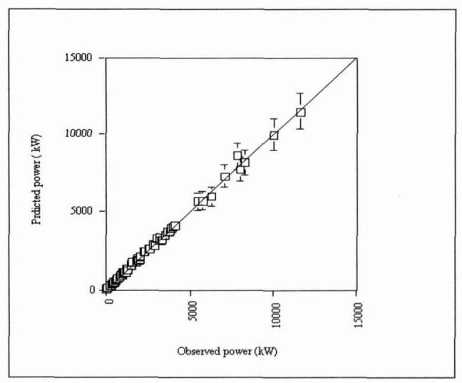
The power draw of a tumbling rnill can be predicted using the equations given below (Morrell, 1996). Their accuracy is illustrated in Figure 2 using data from over 80 ball, ag and sag mills. The 95% confidence intervals are also shown in Figure 2.
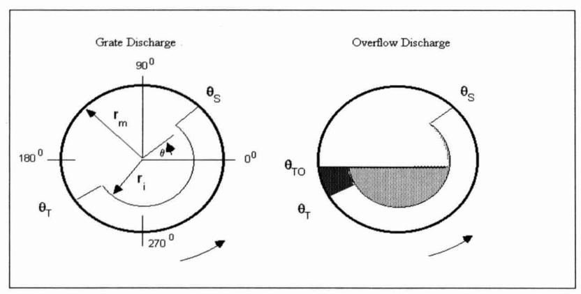
The equations derive from a description of the charge motion based on the simplified charge shapes shown in Figure 3.
gross power = no-load power + (k x charge motion power) (5)
where
gross power = power input to the motor i.e. metered power no-load power = power input to the motor when the mill is empty
charge motion power = power associated with charge motion
k x (charge motion power) = net power
net power = total power input to the charge
In the above, k is a lumped parameter which accounts for heat losses due to internal friction, energy for attritionlabrasion breakage and rotation of the grinding media, plus inaccuracies associated with assumptions and measurements of the charge shape and motion.
Charge motion power for the cylindrical section (P,,) is modelled using the equation:
$$ P_{net} = \frac{\pi g L N_m r_m}{3(r_m - zr_i)} \Big[ 2r_m^3 - 3z r_m^2 r_i + r_i^3 (3z - 2) \Big] $$ $$ + L \rho_c \Big[ \frac{N_m r_m \pi}{(r_m - zr_i)} \Big]^3 \Big[ (r_m - zr_i)^4 - r_i^4 (z - 1)^4 \Big] $$ $$ B = [\rho_c (\sin \theta_s - \sin \theta_t) + \rho_p (\sin \theta_t - \sin \theta_{t0})] $$ (6)
Where the mill has conical ends the power associated with them is given by:
$$ P_{c} = \frac{\pi L_{d}gN_{m}}{3(r_{m} - r_{t})} \left[ r_{m}^{4} - 4r_{m}r_{i}^{3} + 3r_{i}^{4} \right] B $$ $$ + \frac{2\pi^{3}N_{m}^{3}L_{d}\rho_{c}}{5(r_{m} - r_{t})} \left[ r_{m}^{5} - 5r_{m}r_{i}^{4} + 4r_{i}^{5} \right] $$ (7)
No-load power is modelled using the equation:
No-load power (kW) = $$ 1.68D^2(\theta(0.667L_d + L))^{0.82} $$ (8)
where
D = mill diameter
L = length of cylindrical section
L,= length of cone end
8 = fraction of critical speed
p, = slurry density
pc = grinding charge density
010 = angular displacement of the surface of the excess slurry at the toe
gt = angular displacement of the toe of the grinding charge
$$ \theta_t = 2.5307(1.2796 - J_t) \left( 1 - e^{-19.42(\phi_c - \phi)} \right) + - $$ $$ \phi_c = \phi \quad \text{for } \phi \quad > 0.35(3.364 - J_t) $$ (9)
$$ \phi_c = 0.35(3.364 - J_t) $$ for \( \phi \le 0.35(3.364 - J_t) \)
es = angular displacement of the shoulder of the grinding charge =n-(et-0.5)[(0.3386+0.1041$)+(1.54-2.56734)JtI (10) 2
E=fractional porosity of charge
S=fractional solids content (by volume) of discharge slurry U=fraction of grinding media voidage occupied by slurry
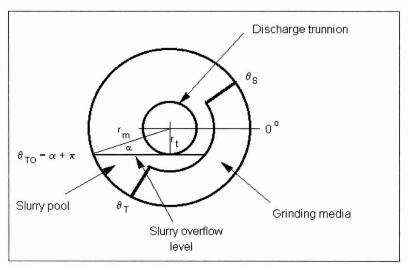
Of particular relevance in the power draw equations is which is the angular position of the excess slurry. Where such slurry exists its effect is to cause a reduction in the power draw - as it does in the case of overflow ball mills when compared to grate discharge ball mills. In an overflow discharge ball mill the level of slurry can be approximated from the geometry of the mill as the slurry must reach the discharge trunnion to exit the mill (Figure 4). Therefore the angular position of the slurry level ( On ) can be estimated quite easily and used in equations (6) and (7). In addition, by definition, the value of U in equation (11) must be equal to unity.
Ag and sag mills use a grate discharge mechanism. In the majority of these mills the slurry level is within the grinding media charge and therefore q, is to equal q,. In mills running under these circumstances when the mill is crash stopped the charge will appear "dry", ie no slurry will be present above the grinding media charge. The parameter U in equation (1 1) will therefore be less than unity. However its exact value is rarely known due to difficulties in its measurement. In these cases the assumption that it is equal to unity is usually sufficient to provide a reasonable prediction of the power draw.
However if the flowrate out of the mill is known the grate flow equations (I) - (4) can be used to estimate U given that it is defined by:
The value of 810 can also be estimated using equations (1) - (4) and simple geometry, as the value of J, reresents the slurry in the pool as indicated by the shaded portions in Figure 3b.
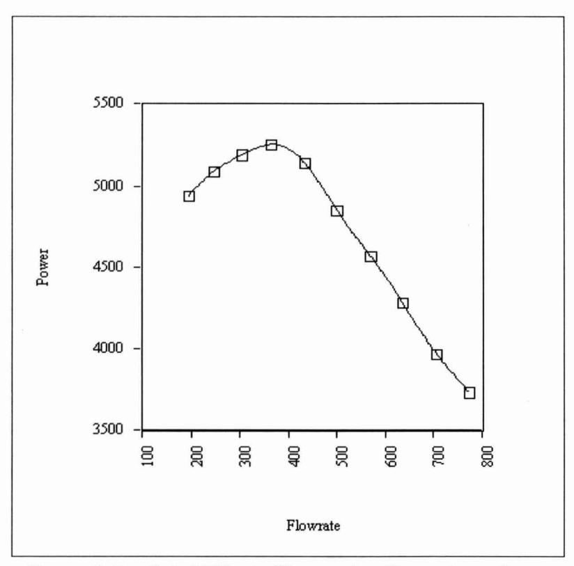
The expected trend in power draw as the slurry flowrate increases can now be predicted using the grate flow and power draw equations. These equations predict that the flowrate-power relationship should be similar to that shown in Figure 5. It can be seen that as flowrate increases the power draw increases at a modest rate until a maximum is reached where all the interstices of the grinding media are occupied. At this point U=l and the charge density ( ) will be at its maximum.
As the flowrate is increased further a slurry pool at the toe forms and is associated with a progressive drop in power draw.
INDUSTRIAL DATA
Given that the power equations described earlier appear to work well in the majority of cases, the power data shown in Figure 6, which were obtained from the Leinster ag mill, are of concern in that in most cases they deviate considerably from the norm. The norm in this case is that predicted using equations (5) - (1 1) under the assumption that there is no slurry pool and U=l. The power data are also given in Table 1 together with the flowrates and associated media fillings which were obtained by crash stopping the mill and measuring the charge levels.
| Data Set | |||||||||
|---|---|---|---|---|---|---|---|---|---|
| Α | В | С | D | Е | F | ||||
| Observed power (kW) | 3,086 | 3,467 | 2,500 | 3,407 | 3,364 | 5,956 | |||
| Expected power (kW) | 4,753 | 5,419 | 3,914 | 4,385 | 3,774 | 6,402 | |||
| Difference (kW) | 1,667 | 1,952 | 1,414 | 978 | 410 | 446 | |||
| Volumetric filling (%) | 20.6 | 24.9 | 16.2 | 18.9 | 15.8 | 32.7 | |||
| Slurry Flowrate (m³/hr) | 581 | 635 | 775 | 740 | 407 | 750 | |||
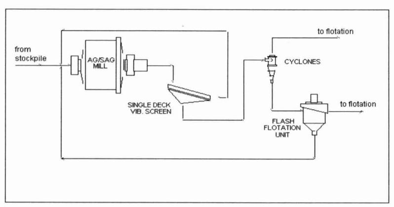
A schematic of the original Leinster circuit is shown in Figure 7. It comprised a single stage ag mill in closed circuit with cyclones and was designed to treat 250 tph (dry) of nickel ore at a final grind p, of 60mm. A more detailed description of the circuit can be found elsewhere (Warder and Davies, 1994).
What was noticeable in all the crash stops apart from the one in which power draw reached 5.956 MW was that excess slurry was present to depths up to about 0.5m.
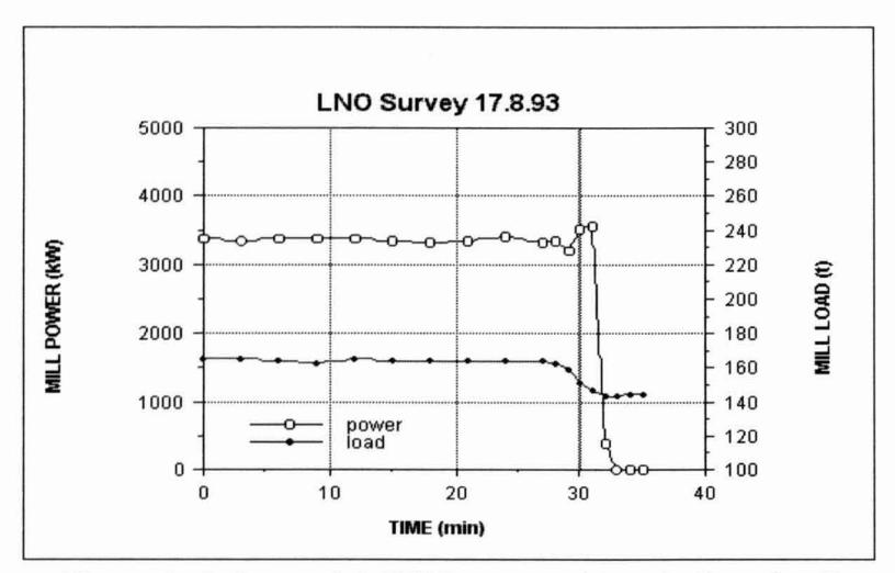
The implication was that slurry pools were forming under some circumstances which were giving rise to low power draws. This was confirmed from investigation of power trends immediately after the feed was turned off. Examples of 2 such trends are shown in Figures 8 and 9. A sharp rise in power is evident in both after the feed is turned off, and in one case reaches almost 1MW above the level just prior to the feed being turned off. This is unusual as a drop in power would be expected due to the drop in mass as the mill ground out. It is hypothesised that under feed conditions a slurry pool was present which caused a low power draw and that immediately after the feed was turned off the slurry pool was rapidly discharged, resulting in a sharp rise in power. As the mill then ground out the power dropped in the usual manner. Further evidence to support this hypothesis comes from 2 other observations. Firstly the magnitude of the power surges shown in Figures 8 and 9 is proportional to the volumetric flowrate.
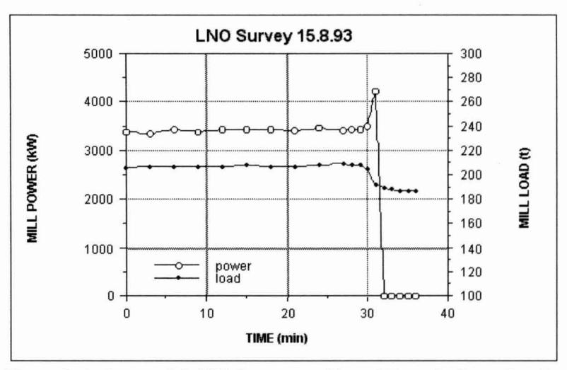
The highest flowrate (and hence highest slurry hold-up) is associated with the largest power surge ie the power draw during normal operation was depressed more. Secondly, data sets A and B were obtained with the original grates which were found to result in excessive blinding and which prompted their redesign. Data sets C, D, E and F were all obtained with the new grates which were much more successful in remaining open. As a reduction in the effective open area of the grates would cause higher hold-ups for the same flowrate it would also be expected that the power draw would be more depressed in normal operation and give rise to a higher power surge when the feed was stopped. This is apparent from the data in Table 1 where the calculated depression in power draw is far greater for the A and B data sets despite the fact their flowrates were lower than in 3 out of 4 of the other data sets.
MODELLING THE POWER DRAW BEHAVIOUR OF THE LEIN-STER MILL
To determine whether the power and grate flow equations could be successfully used to model the behavior of the Leinster mill, the data in Table 1 were used together with the dimensions and grate design data given in Table 2.
| Diameter inside liners (m) | 9.4 | ||
|---|---|---|---|
| Length - belly (m) | 4.94 | ||
| Length - centre line (m) | 6.76 | ||
| Fraction of critical speed | 0.76 | ||
| Grate open area- nominal (%) | 5 | ||
| Grate aperture- nominal (mm) | 15 | ||
It was noticeable that during operation the grate apertures became blocked to varying degrees. This being the case the nominal open area given in Table 2 was never acheived in practice. It was not possible during crash stops of the mill to accurately measure the effective open area of the grates but some photographs of the grates were taken which gave a qualitative assessement of the degree of blinding. For the purposes of this exercise it was assumed that for the data sets C, D, E and F which were associated with the revised grate design the effective open area was 4%. For data sets A and B, which were collected when the original grates were in operation, the effective open area was assumed to be 2%.
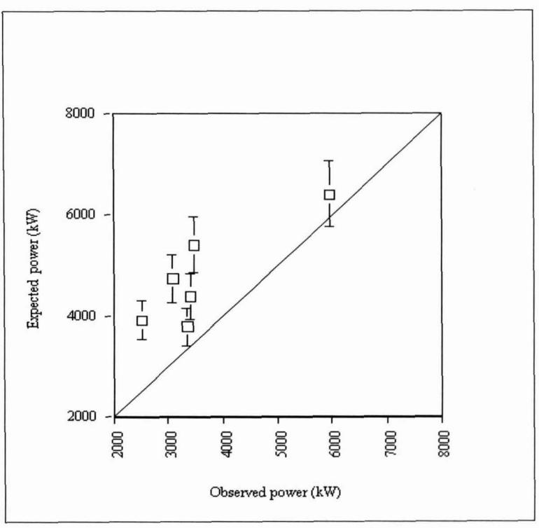
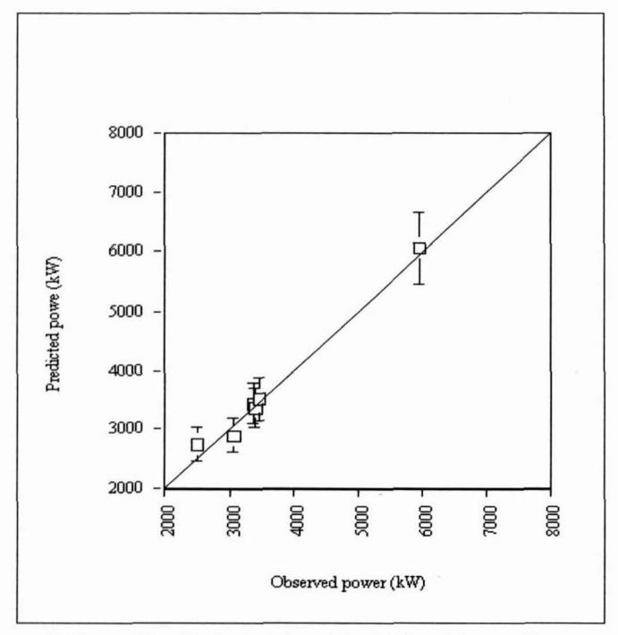
Using these data the slurry hold-ups within the grinding media and at the toe of the charge were estimated from equations 1 and 4. These were then used to estimate and U for each data set. Equations 5-11 were then used to predict the expected power draws. The results are given in Table 3. A graph of the observed vs predicted data is also given in Figure 10. It can be seen that the predicted power draws now match the observed data quite closely.
|
Data
Set |
||||||||
|---|---|---|---|---|---|---|---|---|
| U | 1 | 1 | 1 | I | 1 | 0.84 | ||
| Theta, (rads) | 4.28 | 4.17 | 4.4 | 4.33 | 4.41 | 3.98 | ||
|
Theta,
(rads) |
3.4 | 3.4 | 3.58 | 3.71 | 4.01 | 3.98 | ||
It is interesting to note that only in the case of data set F is there predicted to be no slurry pool. In fact it is estimated that the slurry level resided somewhere below the grinding charge level (U= 0.84) which was observed to be the case from the crash stop. The reason for this was not due to a particulary low flowrate of slurry but was due to the fact that a high volume of grinding media was obtained (32.7% of the mill volume was occupied by grinding media) which was able to contain the hold-up within its interstices. It is no coincidence that data set F was obtained when a particularly competent ore was being treated and that the worst cases of depressed power draw were associated with the treatment of more friable ore.
CONCLUSIONS
It has been observed in a number of cases that as the volumetric flowrate to a mill increases the power draw may drop despite the load continuing to increase in mass.
In such cases the phenomenon can be explained through the build-up of a slurry pool at the toe of the charge which increases as the flowrate increases. The build-up of slurry in this region is associated with insufficient gratelpulp lifter capacity and can be further exascerbated by a relatively low grinding media charge level which results when poorly competent ore is being treated. Using models developed at the JKMRC which relate power draw and flowrate to grinding media and slurry hold-up, this behaviour can be accurately predicted.
ACKNOWLEDGMENT
The support of the sponsors of the AMlRA P9K research project, in particular WMC's Leinster Nickel Operations is gratefully acknowledged. The authors also gratefully acknowledge the permission by
WMC Leinster Nickel Operations and Alcoa of Australia to publish the data relating to their plant.
REFERENCES
Gupta, G K., Hodouin, D and Evereli, M D., 1981. The influence of pulp composition and feedrate on hold-up weight and mean residence time of solids in grate-discharge ball mill grinding. Int. J. Mineral Process , 8 , 345 -358.
Leung K, Lumsdaine I & Veran V P, 1992, Decision of Mount Isa Mines Ltd to change to autogenous grinding, Comminution Theory and Practice , K. Kawatra (ed) pp 331-338.
Morrell S, 1996, Power draw of wet tumbling mills and its relationship to charge dynamics - Part 1: a continuum approach to mathematical modelling of mill power draw. Trans. Instn. Min. Metall. 105. C43 - C53.
Morrell S, 1996, Power draw of wet tumbling mills and its relationship to charge dynamics - Part 2; an empirical approach to modelling of mill power draw. Trans. Instn. Min. Metall. , 105, C54 - C62.
Morrell S, 1989, Simulations of bauxite grinding in a semiautogenous mill and DSM screen circuit. M.Eng. Thesis, University of Queensland.
Morrell S and Stephenson I., 1996, Slurry discharge capacity of autogenous and semi-autogenous mills and the effect of grate design. Int. J. Mineral Process. , in press.
Moys M H, 1986, The effect of grate design on the behaviour of grate-discharge grinding mills. Int. J. Mineral Process , 18, pp 85 - 105.
Warder, J and Davies, M, 1994. Autogenous milling at Leinster Nickel operations. Proc. Fifth mill ops. conf. Roxby Downs, AuslMM 115-121.