Chapter 17

THE PREDICTION OF POWER DRAW IN COMMINUTION MACHINES

S. Morrell and T.J. Napier-Munn Julius Kruttschnitt Mineral Research Centre Isles Road, Indooroopilly, Queensland, Australia

J. Andersen Wimmera Industrial Minerals Horsham, Victoria, Australia

ABSTRACT

The very large quantities of energy used for size reduction in the minerals processing industry necessitate the accurate prediction of comminution machine power draw for optimum plant design. The JKMRC has developed effective models for predicting ball mill, autogenous mill, semi-autogenous mill and crusher power draw. When combined with comminution models they provide a powerful tool for evaluating not only the size reduction performance of a plant design, but its power utilization efficiency as well.

This paper describes the structure of the mill and crusher power models. Data from a wide range of equipment types are presented which illustrate the accuracy of these models.

INTRODUCTION

The energy consumed by comminution equipment in the minerals processing industry accounts for a major part of the operating cost of the plant. Even small improvements to the power utilization efficiency of comminution circuits can therefore have a significant influence on the economic performance of the plant. The application of simulation to explore the energy efficiency of new plant designs and to optimise existing plant therefore has a vital role to play in this regard.

The Julius Kruttschnitt Mineral Research Centre (JKMRC) has been involved with the simulation of comminution and classification circuits for over 25 years. Recently it has developed mathematical techniques for accurately predicting the power draw of ball mills, semi-autogenous mills, fully autogenous mills and crushers, which are reviewed in this paper.

The JKMRC's research activities have generated a large industrial comminution machine data base. This has enabled these power models to be rigorously tested and refined.

THE RELATIONSHIP BETWEEN POWER DRAW AND SIZE REDUCTION

The size reduction action of grinding mills differs from that of crushers. This is due to the differences in the way that power is transmitted by the machine to the ore. The power draw of machines such as jaw and gyratory crushers is dependent upon the ore feedrate and the size reduction across the machine. This in turn is dictated by such factors as the crushing chamber geometry, gap setting, throw and liner profile and condition. Power is drawn "on-demand" when ore particles, which are otherwise too large to pass through the crusher unchanged, are crushed. Power is therefore directly related to the degree of size reduction and hence its prediction must be linked in some way to this process.

The crusher action contrasts with that of grinding mills where the power draw is dictated by the motion and magnitude of the charge. Size reduction can therefore be viewed as a by-product of moving the charge around in the mill. In the case of ball mills in particular, this results in the power draw being largely independent of feed conditions and the amount of size reduction. Modelling of mill power draw can therefore be accomplished without reference to size reduction. Only the motion of the charge needs to be considered.

The following sections will describe the crusher and mill power models in turn. The differences between these machines in their size reduction action is reflected in the very different structure of the models.

THE PREDICTION OF CRUSHER POWER DRAW

The crusher power model enables the prediction of power draw from a knowledge of the breakage characteristics of the ore, the size reduction of ore by the crusher and the relative power utilisation efficiency of the crusher. The breakage characteristics are determined by a laboratory test on representative samples of ore. The power is then predicted from a simple regression equation relating the power actually drawn by the industrial machine in producing a particular product size distribution to the calculated power required to achieve the same size reduction in the laboratory test. The regression coefficients have physical meaning in terms of the power utilisation of particular crusher types and installations. The model was developed by Andersen (1988) based on earlier work by Awachie (1983), and an early version was described by Andersen and Napier-Munn (1988). It has now been applied to several crusher types and has been found to provide satisfactory predictions in each case.

Ore-specific energy - size reduction relationships

The product size distribution of mechanical crushers such as gyratory and cone crushers is dependent mainly on the set or gap, and to a lesser extent on the liner profile and condition, the feedrate and the feed size (Andersen, 1988; Andersen and Napier-Munn, 1990). The power drawn by the crusher to achieve that size distribution under a given set of conditions is then dependent upon the breakage characteristics or "hardness" of the ore.

The breakage characteristics are determined in the laboratory with a single particle twin-pendulum impact device, described by Narayanan and Whiten (1988). This device is used to establish a relationship between the energy used in breaking the particle and the resulting product size distribution. The energy is expressed as the "specific comminution energy", Ecs (units kWh/t), and is calculated from a simple energy balance across the pendulum, and the mass of the particle. The product size distribution is expressed in terms of the t-family of curves described by Narayanan and Whiten (1988), and in particular the t₁₀ parameter. These concepts are an important element in the power model and will therefore be briefly reviewed here.

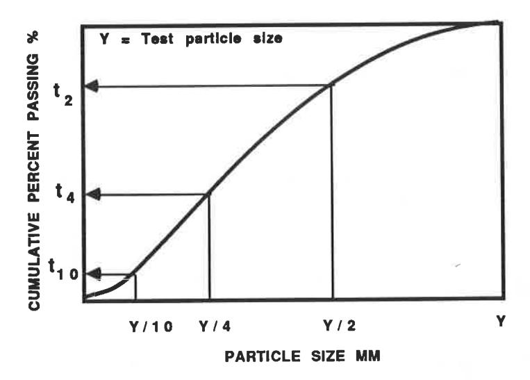
A conventional cumulative size distribution obtained from the breakage of particles of a given size in the twin pendulum can be characterised in terms of the proportion of material passing particular fractions of the initial size of the particles (Figure 1).

The \( t_{10} \) value (the proportion of material passing 1/10 of the original particle size) is usually taken as the characteristic value. By breaking particles with a range of initial sizes at several Ecs values, a range of size distributions and thus \( t_{10} \) values is generated. It has been found if the cumulative percent fineness values are ploted against \( t_{10} \) for other characteristic t-values (such as \( t_{2} \) , \( t_{25} \) , \( t_{50} \) etc.), a family of t-curves results, on which all the initial particle size/Ecs combinations fall (Figure 2).

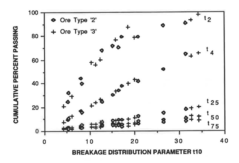
Such a family (or breakage function) is specific to the ore type tested. However the accumulation of a large volume of pendulum data from various sources in recent years has shown that most conventional (brittle) ores can be described by a single family of t-curves, suggesting a common breakage characteristic and further simplifying model prediction algorithms.

The t-curves (eg Figure 2) can be numerically represented by spline functions. If the \( t_{10} \) value for a particular industrial comminution process can be predicted from an appropriate model then the size distribution of the process product can be re-constituted from the spline functions describing the t-curves (ie the breakage function). In the crusher case, the \( t_{10} \) is found to be a characteristic of the particular machine, installation and operating condition.

The final stage in the laboratory breakage characterisation procedure is to establish the relationship between the breakage parameter, \( t_{10} \) , the initial particle size and the specific comminution energy, Ecs, obtained from the pendulum test. Again, these ore-specific relationships can be represented numerically by spline functions.

The Crusher Model

The breakage process in the crusher is described by the well-known Whiten model (Whiten, 1972), which is illustrated conceptually in Figure 3.

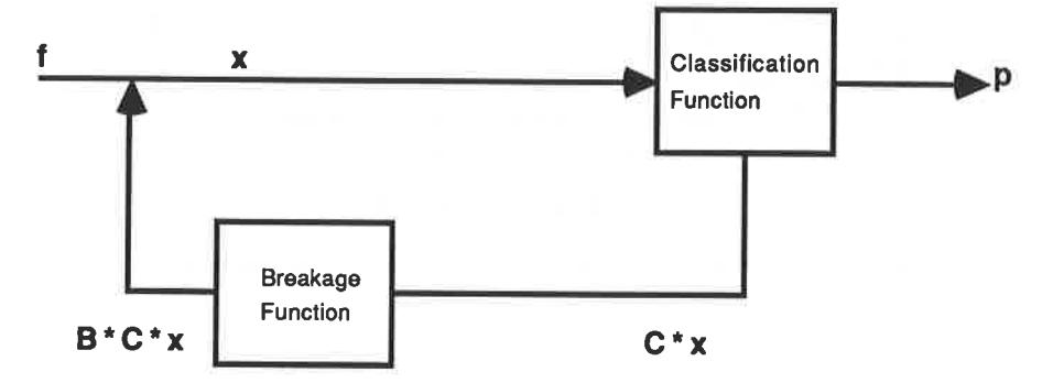
• x is a vector representing the amount in each size fraction in the crusher
• f is the feed size distribution vector
• p is the product size distribution vector
• C is the classification or breakage selection matrix, describing the proportion of particles in each size interval entering the crushing zone
• B is the breakage distribution matrix, giving the relative distribution of each size fraction after breakage.

The product size distribution vector is determined by the mass balance equation

$$ p = (I - C) * (I - BC)^{-1} * f $$ (1)

where I is the unit matrix.

C is a function whose parameters are machine-specific and depend on operating conditions (eg Andersen and Napier-Munn, 1988). The values of the elements in the ore-specific breakage matrix, B, can be determined from the pendulum-derived t-curves.

The values of p are then determined from the spline functions describing the ore-specific t-curves, given the value of \( t_{10} \) . The crusher model, Equation 1, was parameterised so as to fit the three parameters of the classification function, C, and the parameter \( t_{10} \) , to data obtained from plant surveys. Appropriate non-linear parameter estimation techniques were employed. This procedure estimated a value of \( t_{10} \) which best reproduced the data for that particular installation.

In the development of this model, plant surveys of 7-foot (2.13 m) cone crushers were undertaken at Mount Isa Mines (copper ore), Bougainville Copper, Argyle Diamond Mines and Hamersley Iron (Tom Price) (Andersen, 1988). Pendulum tests were conducted on all the feed ores, and a common spline regression was used to represent the resulting t-curves. The t₁₀ parameter was fitted as an installation-specific constant, with values lying in the narrow range 18.3 - 19.9.

The Power Model

The power model relates the actual power drawn by the crusher to the power required by the pendulum to achieve the same size reduction. It is of the form

where

P_C is the power drawn by the crusher under load (kW) P_p is the calculated pendulum power (kW) P_n is the power drawn by the crusher under no load (kW).

Pn is the power drawn by the crusher under no load (kW). A is a dimensionless constant for a particular crusher, obtained by regression

The calculation of the pendulum power, \( P_p \) , is based on the crusher model illustrated in Figure 3. In this model, C is essentially a selection function describing the probability of particles of a given size reporting for breakage. The vector x is the size-by-size mass flow of particles in the crusher (t/h). The product \( C_{ix_i} \) is therefore the mass flow of particles of size i reporting to breakage. When feed and product mass flow and size distribution data are available from plant surveys, and the breakage function B is known from the prevailing value of \( t_{10} \) , then \( C_{ix_i} \) can be calculated by solving the size-by-size mass balance indices in Figure 3. The specific comminution energy, \( E_{Cs_i} \) , appropriate to each size, i, can be obtained from the spline descriptions of the ore-specific \( E_{Cs} \) - \( t_{10} \) -size relationships obtained from the pendulum test. The pendulum power is then given by:

$$ P_p = \sum_{i=1}^{j} E_{cs_{t10i}} \cdot C_i \cdot x_i \quad kW $$ (3)

where

Ecst10i = specific comminution energy at the prevailing value of

t₁₀, for size i (kWh/t)

i = number of size intervals

C_i = probability of breakage of size i

\( x_i \) = mass flow of size i in the crusher (t/h).

\( P_p \) is therefore the total energy required to reduce the crusher feed size distribution to the product size distribution, as if all the reduction took place in the pendulum.

By surveying the same crusher under a variety of power draws and size reductions, it is possible to establish a value for A in Equation 2 by simple least squares linear regression. The parameter A can be interpreted as representing the inefficiency of power utilisation by the crusher (including transmission inefficiencies) compared to that of the pendulum; 100/A is the crusher power efficiency as a percentage of the pendulum power. Power efficiencies in the range 70-80% have been estimated for conventional cone crushers in a variety of mineral processing duties.

Since the power model takes account of the actual size reduction achieved and the tonnage treated by the crusher, it provides a means of comparing the power efficiency of different patterns and types of crusher, in terms of A (or 100/A). The actual power draw of the crusher in a particular duty can of course be estimated by substituting directly in Equation 2 with a value of \( P_p \) corresponding to the duty of interest.

Application of the Model

The power model has been tested in several industrial sites and on several machine types and sizes. In particular, multiple data sets corresponding to a range of operating conditions (particularly feedrate and closed-side setting) were obtained from three sites, all of them operating 7-foot (2.13 m) cone crushers. The crusher type and range of operating conditions studied are summarised in Table 1.

Table 1 - Summary of Industrial Crusher Test Conditions

Site/	Argyle	Hamersley	Mt. Isa Mines
Conditions	Diamonds	Iron	(Copper
		Tom Price**	Concentrator)
Crusher Type	Kobe (A-C)	Nordberg	Nordberg
	Hydrocone	SXHD	SXHD
	EHD5/84	shorthead	shorthead
	with
	Hydroset
Duty	Tertiary	Tertiary	Secondary
Throughput (t/h)	200-710	9-298	180-650
Feed F80 (mm)	35-51	42-77	24-39
CSS (mm)	18-30	14-26	7-12
Throw (mm)	51	111	111
Power draw (kW)	116-378	121-172	180-330
No-load Power	80	117	110
(kW)
No. data sets	18	12	37

Equation 2 was fitted to the industrial data in the form

with A being estimated by linear regression with a suppressed (zero) intercept. The results for the three crushers listed in Table 1 were:

Argyle

$$ P_c = 1.42 P_p + 80 \text{ kW} $$ (s.e. = 0.039; \( R^2 = 0.94 \) )* (5)

Hamersley (Tom Price)

$$ P_C = 1.31 P_p + 117 kW $$ (s.e. = 0.20; \( R^2 = 0.81 \) ) (6)

Mount Isa Mines

$$ P_c = 1.20 P_p + 110 \text{ kW} $$ (s.e. = 0.08; \( R^2 = 0.83 \) ) (7)

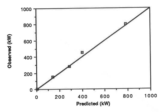
The satisfactory quality of the fits are apparent in Figures 4a - 4c.

Data obtained in joint CSIRO - Hamersley Iron research project; used with permission

^* s.e. = standard error of fitted coefficient

\( R^2 \) = coefficient of multiple determination

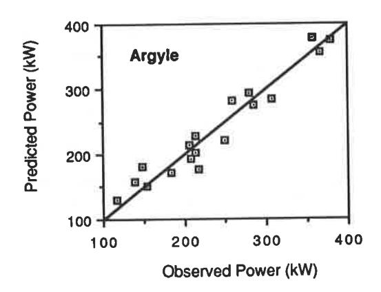
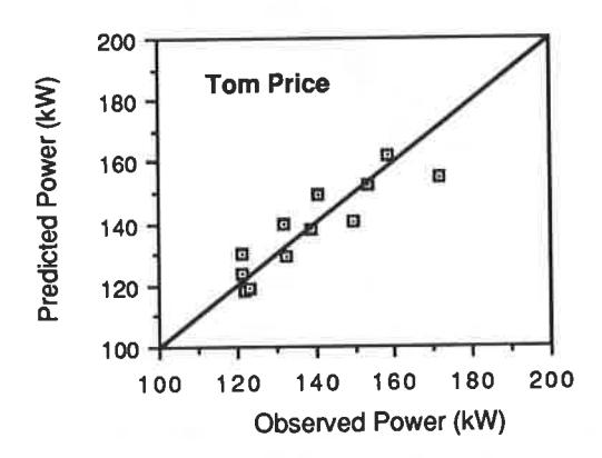
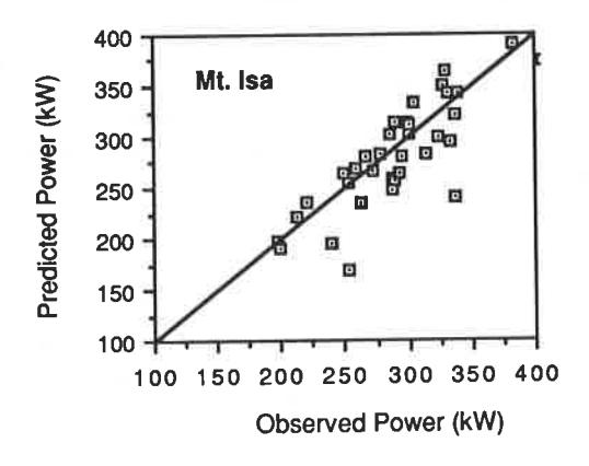
Figures. 4a - 4c - Observed vs Predicted Total Power Draw for Argyle, Tom Price and Mt. Isa Cone Crushers

The values of the coefficients are seen to be similar, the power efficiency (100/A) ranging from 70% to 83%. Statistical tests of the significance of the differences between the estimated coefficients (based on the standard errors of the estimates) suggest that the two shorthead crushers have similar coefficients, but that the Argyle Hydrocone has a significantly higher value than that of the Mt. Isa shorthead. The tests were conducted under very different conditions, and it would therefore be unwise to over-interpret this result. However it may be evidence that the power utilisation efficiency to achieve a given size reduction does depend upon mechanical design.

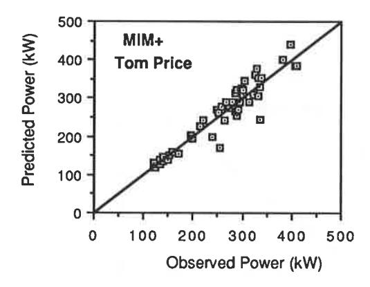
No serious loss in predictive capability is incurred if the mean value of the coefficients for the Tom Price and Mt. Isa SXHD shorthead units is used to represent both machines:

$$ P_{c} = 1.255 P_{p} + \text{no load power} $$ (8)

Figure 5 shows the goodness of fit for the combined data set.

THE PREDICTION OF GRINDING MILL POWER DRAW

A grinding mill draws power to lift its charge of balls and/or ore and to provide it with motion. By describing this motion it is possible to determine the power drawn by a grinding mill for this purpose. Additional power is also drawn to overcome mechanical and electrical losses associated with the mill drive train and bearings. By considering each of these components a prediction of the gross power draw can be made (Morrell, 1991).

Charge Motion

The movement of a charge can be viewed through the end of a laboratory glass mill as shown in Figure 6. By introducing brightly coloured tracers and using photographic techniques, it is possible to measure the position of the toe and shoulder and the velocity of particles at different points within the charge.

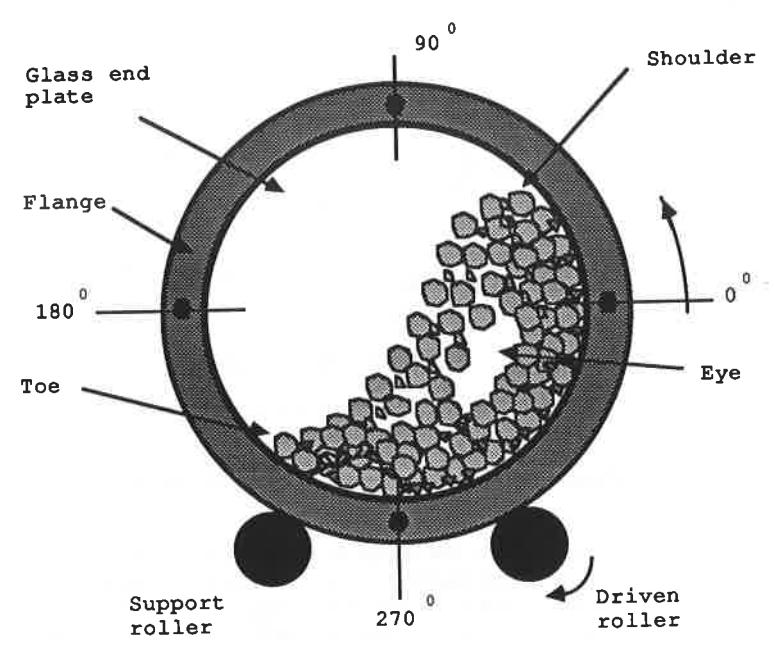
Figures 7 and 8 illustrate schematically how the angular position of the toe and shoulder vary with charge volume and mill speed.

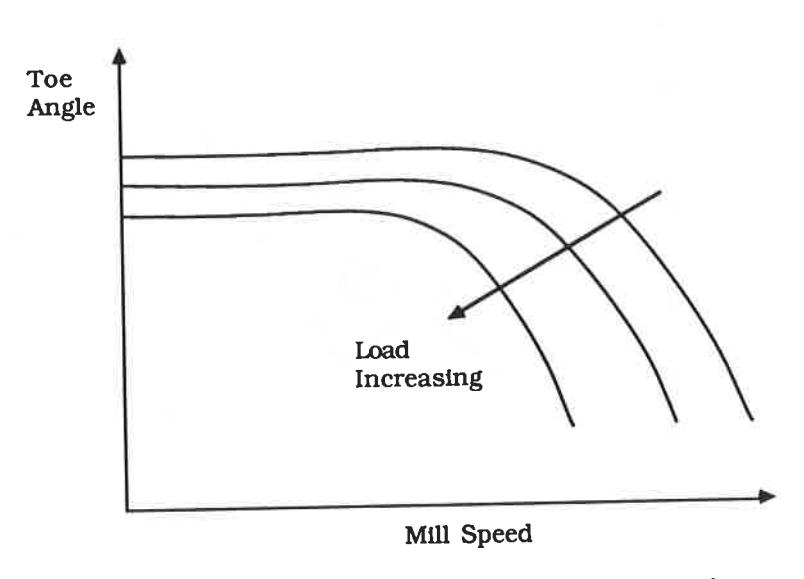
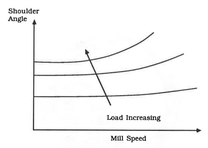
The transfer of energy from the mill shell to the charge is influenced by frictional forces acting on the concentric layers of the charge. The degree of slip between these layers depends on the magnitude of these frictional forces. These in turn are affected by ore type, shape, size and slurry rheology. This can be seen in the charge as a change in angular velocity as the radial position changes.

Particle speeds at different locations were measured from photographs of the mill charge.

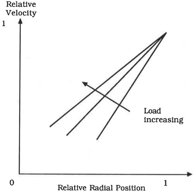
For a wide range of mill speeds tangential velocity was found to be a linear function of radial position with the velocity approaching zero at the eye of the charge. The rate of change of velocity with radial position was also found to vary with mill charge volume (Figure 9).

The Grinding Mill Power Model

The gross power draw of the mill is that drawn by the mill motor(s), ie metered power. It is assumed that this has two components viz.

• net power, ie power delivered to the charge
• no-load power, ie power to overcome drive train and bearing losses.

The gross power can, therefore, be represented by the following equation:

Net Power Draw

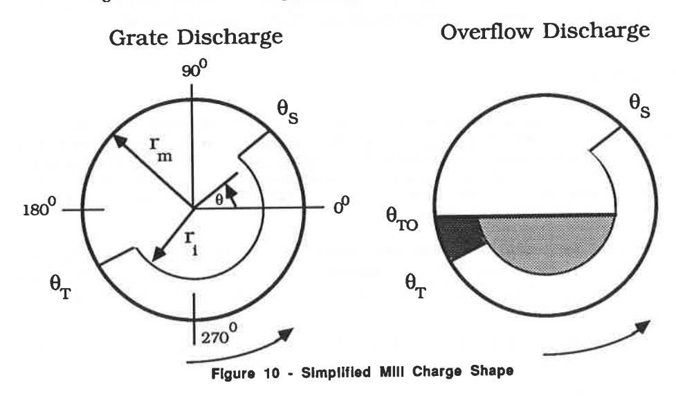
From photographic evidence, charge shapes shown in Figure 10 were assumed to occur in overflow and grate discharge mills. The difference between the charge shape of the two mill types lies in the toe region. In overflow mills there is an additional quantity of slurry represented by the shaded portions in Figure 10. The lighter shaded portion need not be considered as it sits vertically beneath the centre of rotation of the mill. It therefore only contributes a small amount to the weight placed on the bearing and hence the frictional power losses.

By considering an element in the charge of cross sectional area r ds \( d\theta \) and length L the torque inertia of the element can be represented by the following equation:

Torque Inertia of Element = $$ gL\rho r^2 Cos\theta d\theta dr $$ (13)

where

g = gravitational constant

L = mill length

\( \rho \) = charge density

r = radial position of element

\( \theta \) = angular position of the element

Power can be defined in terms of torque \( (\tau) \) and rotational rate (N) as follows:

For grate discharge mills, by integrating between the limits \( \theta_S \) and \( \theta_T \) and between \( r_i \) and \( r_m \) the net power ( \( P_{net} \) ) is given by:

$$ P_{\text{net}} = 2\pi \, \text{gL} \rho \int_{\mathbf{r}_1}^{\mathbf{r}_m} \int_{\mathbf{\theta}_T}^{\mathbf{\theta}_S} N_{\mathbf{r}} \, \mathbf{r}^2 \, \text{Cos} \theta \, d\theta . d\mathbf{r} $$ (15)

where

\( N_r \) = rotational rate at a radial distance r

rm = mill radius

\( r_i \) = charge surface radius (see Figure 10)

\( \theta_s \) = angular position of the shoulder

\( \theta_{\rm T} \) = angular position of the toe.

For overflow mills an additional term must be added to Equation 15 to account for the slurry between positions \( \theta_T \) and \( \theta_{T0} \) (see Figure 10). The density of this portion of the charge will be similar to that of the discharge slurry. The density of the main charge will be different and is estimated from the ore and steel s.g., their relative proportions within the charge, the voidage associated with each fraction and the degree of slurry filling. The value of \( \theta_S \) and \( \theta_T \) are obtained from equations describing the motion of charge of a function of mill speed and charge level (Morrell, 1991).

No-Load Power

The no-load power draw ie that drawn by the mill when completely empty is associated with various electrical and mechanical energy losses. The main ones are motor, gearing and bearing losses. None of these is fixed over the mill's full operating range. Some, however, may have a fixed component. For example, bearing losses due to friction will be dictated by the mill's dead weight (though even this will vary as liners and lifters wear), and the mill charge weight which will clearly vary with grinding condition.

To determine the relationship between no load power and mill design parameters, data from pilot and industrial mills ranging from 1.7 - 7.2 m in diameter were analysed. The parameter \( D^3L \) N was regressed against no load power and found to provide a good fit (Figure 11). The relationship developed was as follows:

No Load Power (kW) = $$ 3.345 (D^3 L N_m)^{0.861} $$ (16)

where

D = mill diameter (m)

L = mill length (m)

\( N_m = mill rotation rate (revs/sec) \)

Model Accuracy

The most recent JKMRC data base currently includes power data from 47 different ball, SAG and AG mills. Details are shown in Table 2.

Table 2 - Mill Data Base Details

Range of Database	Ball Mills	SAG/AG Mills
Diameter (m)	0.91 - 5.5	1.72 - 9.75
Length (m)	1.52 - 8.8	0.58 - 6.6
% Critical Speed	68.5 - 84.0	70.5 - 90.0
% Ball Load	20 - 45	0 - 18
Charge Level (%)	5 7 0.	0 - 45
Gross Power (kw)	7 - 4000	3 - 7000
Ore s.g.	2.6 - 4.5	2.6 - 4.2
No. Mills	26	21
No. Data Sets	31	30

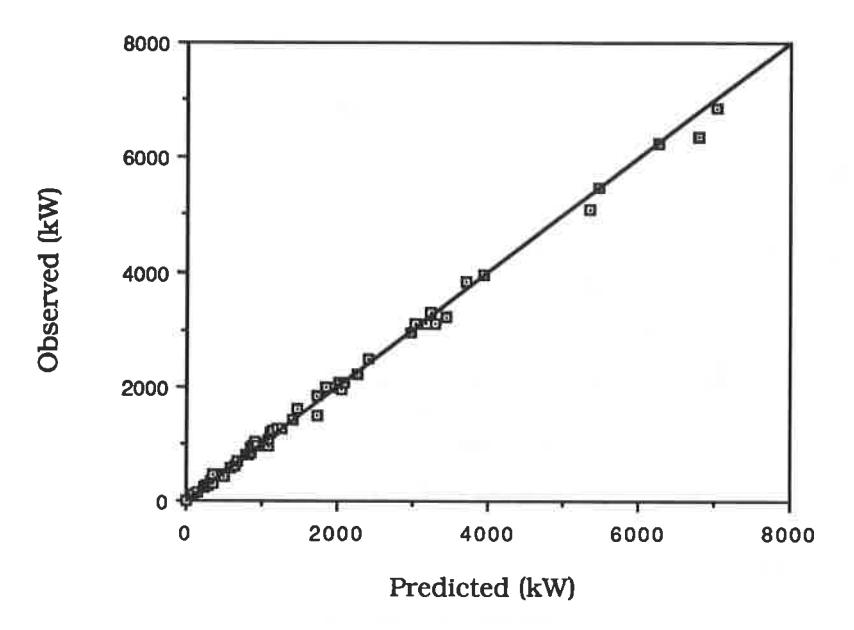
The power model was applied to this data base and found to give excellent results (Figure 12). The standard deviation of the relative error of the model was calculated to be 6.5%.

The model therefore requires a knowledge only of mill dimensions and speed, ball charge, volume occupied by balls and pulp, and the ore specific gravity. Full details of the model are given in Morrell (1991).

CONCLUSIONS - POWER MANAGEMENT IN COMMINUTION CIRCUITS

This paper has described procedures for the prediction of power draw by comminution machines in industrial mineral processing plants. These procedures provide the ability accurately to estimate the total power inventory required for particular circuit configurations, machine sizes and operating conditions, for both existing plants and greenfield designs.

A feature of the techniques, as noted earlier, is the difference in methodologies appropriate for crushers and tumbling mills, which reflects the difference in the way these classes of machine use power to achieve breakage. In crushing, a significant proportion of the power is utilised directly in fracture, and the prediction method must therefore take account of the size reduction being achieved. In ball mills, the majority of power is used to rotate the mill and move the ball charge. The power draw can therefore be accurately predicted without making any assumption at all about the degree of breakage being achieved.

AG and SAG mills fall somewhere between these two cases. The ore component of the charge in such mills, and hence the power used to move it, is significant. Thus a size reduction simulation has to be conducted in order to predict the mass of ore present in the charge.

Despite these necessary differences, there is a strong synergistic effect in bringing together the two computational procedures as tools to analyse the power inventories of particular circuits and to optimise circuit design and machine selection with respect to power draw. An example of such a study was described recently by Morrell et al (1991), in which it was shown that the energy efficiency of a single stage SAG mill/ball mill circuit treating gold ore equalled that of a multistage crushing and milling circuit treating the same ore, but that the latter incurred cost penalties in maintenance and labour; the SAG mill/ball mill circuit was therefore the preferred option.

A common problem in both existing plants and new designs is to optimise the power utilisation between the various classes of machine (crushers, AG/SAG mills, ball mills). In existing plants, this implies making best use of the installed power available. In new plants, a circuit must be designed and equipment selected which will achieve the desired size reduction at minimum project cost. In both cases, the techniques described in this paper, combined with established process simulation methods (eg McKee & Napier-Munn, 1990), offer a powerful tool for the design and optimisation of comminution circuits.

ACKNOWLEDGEMENTS

The work described in this paper was conducted within a JKMRC research project in mineral processing, sponsored by a large number of mining industry companies through the Australian Mineral Industries Research Association. Particular thanks are due to the management and metallurgical staff of Argyle Diamond Mines Limited, Dominion Mining Limited, Hamersley Iron Pty. Limited and Mount Isa Mines Limited, on whose sites data reported in this paper were collected. The authors would also like to especially thank Dr. Keith Weller of the CSIRO Division of Mineral & Process Engineering for permission to use data obtained from the Tom Price tertiary crushers in a joint CSIRO - Hamersley Iron research programme.

REFERENCES

• Andersen J. S. & Napier-Munn T.J., 1988. Power prediction for cone crushers. Proc. 3rd Mill Ops. Conf. , Cobar; Aus. Inst. Min. Met..
• Andersen J.S. & Napier-Munn T.J., 1990. The influence of liner condition on cone crusher peformance. Minerals Eng. , Vol. 3, No. 1/2, 105-116.
• Andersen J.S., 1988. Development of a cone crusher model. M Eng (Sc) thesis, University of Queensland.
• Awachie S.E.A., 1983. Development of crusher models using laboratory data. PhD thesis, University of Queensland.
• McKee D.J. & Napier-Munn T.J., 1990. The status of comminution simulation in Australia. Minerals Eng. , 3, No. 1/2, 7-22.
• Morrell S., 1991. The Prediction of Grinding Mill Power. Accepted for publication in Trans. Inst. Min. Met.
• Morrell S., Johnson G. & Revy T., 1991. A comparison through observation and simulation of the power utilization performance of two dissimilar comminution plants. Proc 4^th Mill Operators Conference, Burnie, Tasmania; Aus. Inst. Min. Met.
• Narayanan S.S. & Whiten W.J., 1988. Determination of comminution characteristics from single particle breakage tests and its application to ball mill scale-up. Trans. Inst. Min. Met. , 97, C115-C124.
• Whiten W.J., 1972. The simulation of crushing plants with models developed using multiple spline regression. J.S.A. Inst. Min. Met., 72, 257-264.