



The content on this page was automatically generated from the PDF publication document and may contain errors or inaccuracies. Please refer to the original PDF for the most accurate information.
THE PREDICTION OF POWER DRAW IN WET TUMBLING MILLS
Stephen Morrell B.Sc (Eng), M.E.
Thesis submitted in fulfillment of the requirements for the degree of Doctor of Philosophy
Julius Kruttschnitt Mineral Research Centre Department of Mining and Metallurgical Engineering University of Queensland
ABSTRACT
The last 90 years have generated a considerable volume of technical literature on the subject of grinding mill power and its prediction. It is therefore surprising that in all this time there have been no published models for predicting grinding mill power draw which have been validated using a published wide range of comprehensive industrial scale data.
Notwithstanding this lack of data, the majority of models have placed limited emphasis on the internal dynamics of mills and have relied on simple assumptions which consider the charge to take up a fixed position and shape. In recent years laboratory based studies (Liddell, 1986) have shown that these assumptions do not hold over a wide range of operating conditions, and bring into doubt the ability of existing models to accurately predict grinding mill power draw.
To remedy this deficiency a research programme was therefore undertaken to:
- provide a large compehensive data base of the power draws of industrial scale ball, semi-autogenous (SAG) and autogenous (AG) mills
- use these data to develop mathematical models which can accurately predict the power draw of industrial grinding mills over a wide range of operating and design conditions
The approach which was adopted utilized a glass fronted laboratory mill, operating under a range of speeds and fillings, to provide data on the movement of a charge in a grinding mill. The position of critical points in the charge and the velocity of particles within the charge were measured with the aid of photographic techniques. These measurements were then related mathematically to the operating conditions using empirical techniques.
The equations which were developed from this exercise were incorporated in a theoretical approach to the prediction of power draw. The resultant model explicitly described the effects of the mill discharge mechanism (i.e. grate or overflow), as well as the shape of the end sections (i.e. planar or conical). The model made no specific distinction between ball, semi-autogenous (SAG) or autogenous (AG) mills except by virtue of their charge density and/or discharge mechanism. Two further models were developed, one of which was more complex in nature but which additionally accounted for the effect of grinding media size distribution on power draw. The other model was an empirical version with a very simple form yet similar predictive performance to the other two.
Data were collected from a wide range of wet industrial grinding mills to calibrate and verify the model. In total 76 data sets were generated covering the power draws of ball, SAG and AG mills in the range 7 - 7900 kW. All three models were found to predict the power draw of the mills in the data base with a high degree of accuracy. This contrasted with the results from testing a number of existing published models, none of which were found to be entirely satisfactory.
STATEMENT OF ORIGINALITY
I declare that the work presented in this thesis is, to the best of my knowledge and belief, original, except as acknowledged in the text, and that the material has not been submitted, either in whole or in part, for a degree at this or any other university.
Signed:
Stephen Morrell
Date: 27th July 1993
LIST OF PUBLICATIONS
Following is a list of the author's published technical papers on the subject of power draw and grinding:
- Lynch A.J. and Morrell S., 1992. The understanding of comminution and classification and its practical application in plant design and operation. Comminution - Theory and Practice , K. Kawatra (ed), SME, Ch 30, pp 405 - 426.
- Morrell S., Johnson G. and Revy T., 1991. A comparison through observation and simulation of the power utilization performance of two dissimilar comminution plants. Proc. 4th Mill Operators Conference , Burnie, Tasmania, Austral. Inst. Min. Metall.
- Morrell S., 1992. The simulation of autogenous and semi-autogenous milling circuits. Comminution - Theory and Practice , K. Kawatra (ed), SME, Ch 27, pp 369 - 380.
- Morrell S., Napier-Munn T.J. and Andersen J., 1992. The Prediction of Power Draw in Comminution Machines. Comminution - Theory and Practice, K. Kawatra (ed), SME. Ch 17, pp 235-247.
- Morrell S., 1992. Prediction of grinding mill power. Trans. IMM , Vol 101, C 25 - 32.
- Morrell S., Sterns U.J. and Weller K.R., 1993. The Application of Population Balance Models to Very Fine Grinding in Tower Mills. Proc. XVII Int. Min. Processing Congress , Sydney, Austral. Inst. Min. Metall., Vol 1, pp 61-66
- Morrell S., Dunne R.C. and Finch W., 1993. The Liberation Performance of a Grinding Circuit Treating Gold Bearing Ore. Proc. XVII Int. Min. Processing Congress , Sydney, Austral. Inst. Min. Metall., Vol 1, pp 197- 202
ACKNOWLEDGEMENTS
I would like to acknowledge the following people for their contributions, both directly and indirectly, to the preparation of this thesis.
- Dr. D.J. McKee and Dr. T.J. Napier-Munn, for their enthusiastic support throughout my studies, and in particular for their suggestions about the structure of this thesis.
- Dr W.J. Whiten, my academic supervisor, for his general guidance, encouragement and suggestions on the structure of the thesis. In particular, I would like to thank him for his advice on the use of tracers and on photographic technique when studying the glass laboratory mill.
- Justin Scowen for his assistance with taking some of the photographs of the glass laboratory mill.
- • Staff and students of the P9J/P9K mineral processing research team and JK Tech who assisted with collecting industrial grinding mill data, in particular Bill Finch and Dr Toni Kojovic.
- The sponsors of the AMIRA P9J/P9K research programme for their support and cooperation, particularly with regard to the unrestricted access to their treatment plants and data.
- Bob Pendreigh for his kind and valuable donation of the data he collected when dumping and analyzing a mill charge at the Union Corporation of South Africa.
- Debbie Farmer and Fern Ausland for typing and laying out the thesis.
- My parents for their influence, particularly in my formative years, and for their never-failing interest and support throughout my life.
- My children, Andrew, James and Lauren who, uncomprehendingly, have sometimes felt the brunt of my bad temper, borne of the frustrations of this thesis. To them I apologize.
I would like to make a very special acknowledgement to my wife, Leana. No words that I can write here can do justice to the support she has given me in my studies, nor the physical effort she has put into making up for my lessened contributions to running our household whilst preparing this work. I am eternally grateful.
Lastly, though by no means least, I would like to thank God.
CHAPTER 1
INTRODUCTION
1.1. THESIS ORIGINS
The origins of this thesis lie in mid 1987 when the author started Master of Engineering studies into semi-autogenous (SAG) and autogenous (AG) mill modelling. One of the outcomes of these studies was the realization that, ideally, data on both the charge mass and charge size distribution were essential to understand and model the grinding behaviour of SAG and AG mills (Morrell, 1989).
In practice obtaining both the mass of the contents of a full scale industrial mill and sizing it is both time consuming and expensive. This difficulty is reflected in the very few published cases where this task has been undertaken (Stanley, 1974; Morrell, 1989). Although not ideal, knowledge of only the mass of the charge in a mill can be used to advantage in fitting of model parameters in simulations of SAG/AG mill circuits (Lynch and Morrell, 1992; Morrell, 1992). In studying industrial mills, however, it is quite often the case that production constraints do not allow for mill stoppages to measure charge levels and hence determine charge masses. This usually leaves only the power draw of the mill as an indication of what the mass of the contents of the mill is. This limitation in studying industrial mills suggested the potential use of equations for predicting power draw as a means of back-calculating the mill charge mass from observed power draw data.
Coincidentally, at about the same time a number of mill operators sponsoring the Julius Kruttschnitt Mineral Research Centre's (JKMRC) mineral processing research programme, expressed dissatisfaction with both published models, and manufacturers' estimates of SAG/AG mill power requirements. Their request of the JKMRC was to develop a model which could be used both for design of SAG/AG milling circuits and to assist in optimising existing installations. Of particular interest in regard to this latter requirement was the ability to predict under what conditions peak power draw occurred.
The need in SAG/AG modelling work of at least a charge mass estimate, and the perceived (by mill operators) deficiencies of existing power prediction models, therefore lead to the initiation of a research programme in this area.
1.2 OBJECTIVE OF THESIS
Although the needs of both the JKMRC research sponsors and its own in-house research was focussed on SAG/AG mills, it was decided to extend the research to cover all wet grinding mills using rock and/or ball grinding media. Rod mills were not included due to the rapidly dwindling number of installations in Australia.
The objectives of the thesis, therefore, were as follows:
- i) To provide a large, comprehensive and relatively accurate data base of industrial ball, SAG and AG mills for use in studying power draw.
- ii) To develop a model which can be used to accurately predict the power draw of industrial ball, SAG and AG mills.
1.3 STRUCTURE OF THESIS
The thesis is organized into 9 chapters, including this introduction. Chapter 2 reviews published literature on power prediction equations/models, highlighting both the similar approach used in most of the techniques and the apparent lack, in most cases, of any industrial data to confirm that the techniques apply to industrial mills.
In Chapter 3 the groundwork for the development of a power model is laid by developing relationships for the shape and motion of the charge in a glass laboratory mill under a range of fillings and speeds. The equations developed in Chapter 3 are incorporated in Chapter 4 in a theoretical approach to describing the power draw of a simple cylindrical batch tumbling mill operating under wet conditions.
Chapter 5 extends the equations describing the theoretical power draw of simple batch mills to conditions which cover the variety of mill designs and operating conditions found in wet industrial grinding mills (C-model). The data collected on such mills are given and described in Chapter 6 with particular reference to the data diversity and the problems with obtaining accurate data.
In Chapter 7 the C-model is calibrated using the data base and its accuracy evaluated using a variety of techniques. At the same time a number of published models are evaluated and compared with the C-model. A new semi-empirical model is also presented (E-model) whose performance is partly based on that of the C-model. In conjunction with the data base, the E-model is used to determine the exponent which most closely describes the diameter relationship with power in grinding mills.
In Chapter 8 a third model (D-model) is described. Due to the limited data on load size distributions that this model requires for calibration, and its somewhat different approach to power draw modelling, its description, calibration and validation is given in a separate chapter at the end of the thesis. Its structure is based on a more detailed description of the charge motion in which the charge is considered to comprise a series of layers or shells. This approach is shown to account for grinding media size effects on power draw - effects which are not specifically addressed by either the C or E models. In addition, its use in making tentative conclusions concerning the contribution of impact breakage and attrition/abrasion breakage is also described.
Chapter 9 completes the thesis by summarizing the main conclusions and makes recommendations for further research.
Throughout the thesis, symbols have been defined locally. In addition a list of the symbols used in the author's equations is given in the Nomenclature.
CHAPTER 2
LITERATURE REVIEW
A review of literature on the subject of mill power draw predictions has been undertaken as far back as 1905. It was found that numerous models for predicting mill power have been published, yet none were provided with comprehensive full scale mill data to prove their practical applicability. Bond's equation (1961/62) was claimed by Bond, Rowland (1972) and Kjos (1979) to be based on full scale ball mill data. Unfortunately, none of their data were ever published in full.
The relatively recent popularity of SAG and AG mills has resulted in few power models which relate to the power consumption of these mills. Austin's model (1990) purports to have been specifically designed for SAG mills, though not for ball mills. The only general model form has been put forward by Harris et al (1985), which claims to predict the power draw of ball, SAG and AG mills.
Although many mill power models have been proposed, most have the same form or are derivatives of the same form. Only the discrete element method approach of Mishra and Rajamani (1990) can be said to represent, in more recent times, a truly different way of predicting mill power draw.
2.1 INTRODUCTION
The literature contains a large number of publications relating to the power draw of grinding mills, either from an academic modelling or from an operational/design viewpoint. A common denominator in all of them is a lack of any substantial wide ranging industrial data. As the purpose of this literature review is to discuss the status of research into the prediction of mill power draw, this lack of published reliable data has resulted in little critical evaluation of the validity of the techniques and assumptions that previous researchers have used.
To provide a literature review which is comprehensive, yet at the same time is useful and focuses on the limitations in the status-quo of research in this field, a core of what is considered to be the principal pieces of research effort over the last 100 years has been chosen for detailed commentary. Given the lack of substantial supporting data in all published work, the review largely confines itself to the presentation of the techniques and assumptions that have been adopted by the various researchers. In Chapter 7, however, the industrial mill data base, generated from the research programme described in this thesis, is used to evaluate a number of published power models.
2.2 DEVELOPMENTS IN GRINDING MILL POWER MODELLING IN THIS CENTURY
2.2.1 Overview
Table 2.1 chronologically lists the more significant developments in grinding mill power modelling since the turn of the century. Two criteria were used to compile the table, viz:
- does the development approach the problem in a different manner?
- does the development relate to a particular area of grinding mill power prediction not previously covered?
The result is a list of 11 pieces of work, a summary of which is also given in Table 2.1. Each of the 11 works is reviewed in the following sections. A list of additional papers related to the subject of grinding mill power draw is given in Appendix 5.
| Date | Author | Development |
|---|---|---|
| 1919 | Davis | On the basis of a theoretical treatment of the motion of particles |
| in a mill under the influence of gravity and centrifugal force, a | ||
| mill power equation was developed which predicted the power | ||
|
draw at the 'optimum speed'.
This speed was defined as that |
||
| which maximized the impact velocities of particles. | ||
| 1956 | Rose and Evans | Using an instrumented drive mechanism, the effect of a wide |
| range of design and operating variables was determined | ||
| experimentally using mills with diameters less than 3 inches. A | ||
| power draw equation was subsequently developed based on | ||
|
dimensional analysis.
They applied these models to Taggart's |
||
| data. The model gave the same trends as observed in Taggarts | ||
| data but with a fair degree of scatter. | ||
| 1961/62 | Bond | Developed a semi-empirical ball mill equation using industrial |
|
data
(unpublished) and laboratory based experiments |
||
| (unpublished). | ||
| 1972 | Hogg and | Used a simplified description of the charge shape in which it was |
| Fuerstenau | assumed that there existed an equilibrium surface defined by the | |
| chord joining the toe and shoulder; the angle of repose of the | ||
| charge was assumed constant over all conditions. On the basis of | ||
| this description they developed a power equation by considering | ||
| the rate at which potential energy was imparted to the particles | ||
| in such a charge. | ||
| 1982 | Arbiter and Harris | Used the same charge assumptions as Hogg and Fuerstenau and |
| developed a power equation based on torque-arm principles. | ||
| The resultant equation was essentially identical to Hogg and | ||
| Fuerstenau's. The equation was fitted to Taggart's data to enable | ||
| the mean angle of repose of the charge to be determined. No | ||
| results were provided on how the model fitted these data. |
| 1985 | Harris, Schnock |
Developed
'correlation equations' whose parameters were |
| and Arbiter | determined on the basis of equipment suppliers models and | |
|
data.
Their equation was a generalised form whose structure |
||
| reflected the equations of Bond, Hogg and Fuerstenau and their | ||
| earlier equation from 1982. A major conclusion of this work was | ||
| that there existed a lack of reliable published data which could | ||
| be used to verify/develop accurate mill power equations. | ||
| 1986 | Liddell | Conducted experiments using a 0.55 x 0.3m laboratory mill to |
| determine the change in shape of the charge inside a mill under a | ||
| range of mill fillings, speeds and slurry rheologies. From torque | ||
| measurements of this mill he also related power draw to these | ||
| conditions. From the results of these experiments he concluded | ||
| that the equations of Bond, Hogg and Fuerstenau, and Harris | ||
| and Arbiter did not adequately reflect the observed power draw | ||
|
of his mill over the full range of speeds he used.
He |
||
| subsequently modified Harris et al's equation and incorporated a | ||
|
tabulated
speed correction function which matched his |
||
| observations of the effect of speed on power draw. The model | ||
| was not applied to industrial data. | ||
| 1990 | Fuerstenau, Kapur | Considered that the charge in a mill comprised 2 parts, viz. a |
| and Velamakani |
cataracting fraction and a cascading fraction.
The cascading |
|
| fraction was assumed to be adequately described by the Hogg | ||
| and Fuerstenau equation. The cataracting fraction was assumed | ||
| to be subject to viscous forces and was described separately | ||
| using a torque-arm based equation. The relative magnitude of | ||
|
the cataracting fraction was related to slurry viscosity.
The |
||
| model contained at least 6 parameters which were fitted to batch | ||
|
laboratory ball mill data.
The model was not applied to |
||
| industrial data. |
| 1990 | Moys |
Also assumed that the charge comprised 2 parts, viz. a
centrifuging layer and a non-centrifuging fraction. The non |
| centrifuging fraction was assumed to behave in a manner which | ||
|
Bond's
equation, without its speed correction function, |
||
| adequately described. The centrifuging fraction was assumed to | ||
| be affected by lifter configuration/design and slurry viscosity, | ||
| such that it would tend to centrifuge in advance of the remainder | ||
| of the charge as the mill speed increased. The relative magnitude | ||
| of this fraction was modelled empirically. The parameters of the | ||
| model were fitted to data from a 0.55 x 0.3m laboratory mill. The | ||
| model was not applied to industrial data. | ||
| 1990 | Austin | Developed a model specifically for predicting the power draw of |
| SAG mills. Hogg and Fuerstenau's equation was used as a basis | ||
|
for the model.
It was modified by Austin to incorporate the |
||
| energy used to provide kinetic energy to the charge plus the | ||
| power consumed by the charge in the conical ends of the mill | ||
|
(where fitted).
To account for the reduction in mill power |
||
| observed beyond a certain speed he added Bond's empirical | ||
| speed correction factor. Finally he modified the density term in | ||
| the equation to reflect the ball/rock/slurry mix in SAG mills. He | ||
| fitted his model to published data on 2 industrial mills. | ||
| 1990 | Mishra and | Used discrete element methods to describe the motion of balls in |
| Rajamani | a ball mill. The code was modified to provide the theoretical mill | |
| torque based on the shear forces exerted on the mill shell. They | ||
| used the data from Liddell and Moys' 0.55 x 0.3m mill to validate | ||
| their model. The model was not applied to industrial data. | ||
2.2.2 Davis
Davis (1919) appears to be the first person to attempt to relate ball charge motion in a mill to its power draw. It is not possible to tell whether Davis developed his physical and mathematical description of the ball charge motion independently or used the much earlier and similar work of White (1905), which Richards (1909) claimed was the best piece of research on charge motion of the time. Davis, in his paper, did not reference any other research. White generously gave Davis the benefit of doubt and commented that Davis did not do so due to "... neglect of the usual distinction between ball and tube mills". Davis, however, does use the same description of the charge motion as White, in which the particles move in a locked manner in a circular path until a point is reached where the centrifugal and gravitational forces balance. At this point particles commence free fall in a parabolic path until they impact the mill shell and start their circular path once more. Frictional forces and interparticle interference were ignored.
Using this approach Davis calculated the point at which particles commenced and terminated their parabolic free fall. For the commencement of free fall the locus was given by a circle of radius g/2ω2 whose centre was vertically above the centre of rotation of the mill at a distance of g/2ω2 (Figure 2.1).
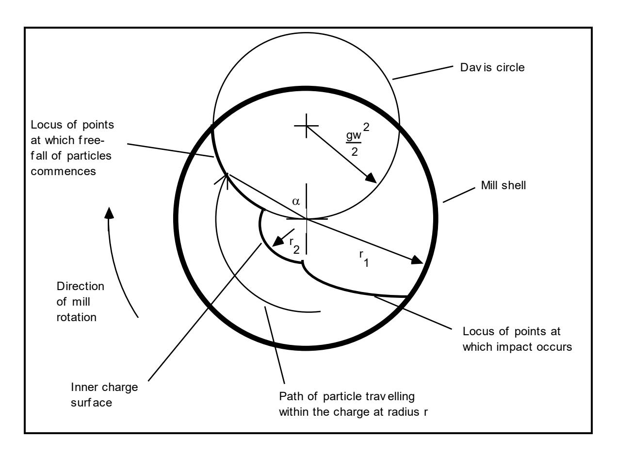
The co-ordinates of the point of impact were calculated to be:
From these equations, the kinetic energy of particles when they impacted the mill shell at the end of their free-fall was computed as follows:
$$ e = w(8Fr^2 - 16F^3r^4 + 8F^5r^6) $$ (2.3)
where
e = kinetic energy
w = weight of any particle
F = 1.226n2
n = mill speed in revs per sec
r = radius of circular path.
Equation 2.3 was then integrated between the radial limits of the charge (r1 and r2). The inner radius (r2) was related to the mill radius (r1) using the expression:
The term K was the fraction of the mill volume which was occupied by that part of the charge not in free flight. K was related to the fraction of the mill volume which was occupied by the charge when stationary (P), as follows:
$$ K = -0.024 + 0.39\sqrt{7-10P} $$ (2.5)
Davis chose to arrange his power equation in terms of the 'most efficient speed'. This was defined as the theoretical speed at which the particle kinetic energy on impact was maximized. His equation was therefore given as:
Mill Power (hp)
$$ = Wr_1^{3/2} \left[ 0.004467 \frac{(1-K^3)}{(1+K^2)^{1/8}} - 0.0037 \frac{(1-K^5)}{(1+K^2)^{3/8}} + 0.00088 \frac{(1-K^7)}{(1+K^2)^{5/8}} \right] $$ (2.6)
where
\( r_1 \) = mill radius in feet
W = weight of charge in pounds.
Davis claimed that the equation was valid only for mills operated at the most efficient speed (N). N was defined by the following equation:
$$ N = \frac{48.948}{r_1^{0.5} (1+K^2)^{0.25}} $$ (2.7)
Davis conducted experiments using a 3 inch diameter mill and stated that his idealized charge motion was observed in practice. He did not, however, provide any evidence that his formulae successfully predicted the power draw of industrial mills.
2.2.3 Rose and Evans
The contributions of the work conducted by Rose and Evans are reported in the first 2 papers in a trilogy written between 1954 and 1955 and published in 1956 (Rose and Evans, 1956; Rose and Blunt, 1956).
The work of these 2 researchers was the first, and so far as can be seen, remains the most thorough investigation of most of the factors which might reasonably be expected to affect grinding mill power draw. The work was conducted using mills of less than 3 inches in diameter.
Dimensional analysis was used to develop the following equation:
$$ \frac{\left(\underline{\sigma}\right)}{\rho}, \left(\underline{L}\right), \left(J\right), \left(f\right), \left(e\right), \left(v\right), \left(u\right), \left(n\right) $$ (2.8)
where h a representative particle dimension D internal diameter of the mill d diameter of the balls e coeff. restitution between the balls and the mill acceleration due to gravity g Н energy required to bring about unit increase in the specific surface of the powder (specific surface in units of area per unit mass) h height of lifters Ţ volume occupied by the ball charge (including voids), expressed as a fraction of the mill volume T. internal length of the mill N speed of rotation of the mill, rev per sec \( N_c \) critical speed of rotation of the mill number of lifters n Р = power denotes some function of each of the dimensionless groups φ = volume occupied by fluid expressed as a fraction of u the volume of voids in the charge volume occupied by the powder charge (including voids), v expressed as a fraction of the volume of voids in the ball charge density of ball material ρ ν kinematic viscosity of the mixture of powder and fluid effective density of the mixture of powder and fluid. σ
To simplify equation 2.8, the dimensionless groups relating to the characteristics of the powder and fluid were omitted. The relationships between the remaining groups and the power number were then determined experimentally and presented in graphical form.
For a mill containing a ball charge only, Rose and Evans found that equation 2.8 could be reduced to the following form:
$$ \frac{P}{D^5 N^3 \rho} = \left(\frac{L}{D}\right) \times \phi_1 \left(\frac{N_c}{N}\right) \times \phi_3 \left(J\right) \times \phi_4 \left(\frac{D}{d}\right) \times \phi_5(n) \times \phi_6 \left(\frac{h}{D}\right) $$ (2.9)
When powder was introduced they found that the functions \( \phi_3 \) and \( \phi_4 \) were different. These were represented in notational form by \( \phi_3 \) and \( \phi_4 \) . In addition the form of equation 2.9 needed to be modified as follows:
$$ \frac{\rho}{D^{5}N^{3}\rho} = \left(1 + 0.4 \frac{\sigma}{\rho}\right) \left(\frac{L}{D}\right) \times \phi_{1} \left(\frac{N_{c}}{N}\right) \times \phi_{3}' \left(J\right) \times \phi_{4}' \left(\frac{D}{d}\right) \times \phi_{5} \left(n\right) $$ $$ \times \phi_{6} \left(\frac{h}{D}\right) \times \phi_{9} \left(\frac{D}{b}\right) \tag{2.10} $$
A further modification was introduced to account for observed differences between grate and overflow mills. This was done by the incorporation of a correction factor. The calculation route for determination of the correction factor was not provided, only a graph of the variation in its value with powder density and ball filling. It was stated, however, that the correction factor was calculated by considering the moment (torque) of the powder layer between the ball charge level and overflow trunnion.
In most practical situations some of the terms in equation 2.10 were found to tend to unity. Hence equation 2.10 reduced to:
$$ \frac{P}{D^5 N^3 \rho} = \left(1 + 0.4 \frac{\sigma}{\rho}\right) \left(\frac{L}{D}\right) \times \phi_1 \left(\frac{N_c}{N}\right) \times \phi_3' \left(J\right) $$ (2.11)
It was found that for N < 0.75 \( N_c \) and a mill with lifters, the speed function ( \( \phi_1 \) ), could be approximated as follows:
The relationship between J and φ3' (J) was as shown in Figure 2.2 and shows a peak in the function at J = 0.4. This reflects their observed experimental maximum in mill power draw as the mill filling was increased.
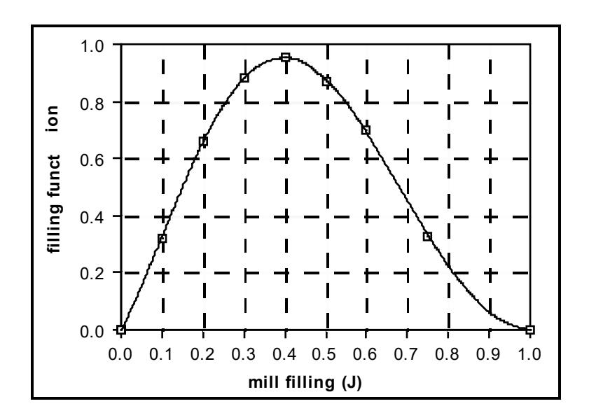
The authors applied their model to a dual compartment ball mill 6 feet in diameter and 22.5 feet long. They found that their formulae under-estimated the power by about 20%. This they attributed to meter and drive train inefficiencies. Using a range of inefficiencies of 15 - 25%, they also applied their model to Taggart's data (Taggart, 1945). It indicated similar trends but with a fair degree of scatter.
Interestingly, although the effect of changing ball size was examined by Rose and Evans, the conclusion drawn was that ball size had little effect. Bond (1956), whilst praising the work, criticized this aspect as having not gone far enough. This was on the basis that in industrial mills a decrease in ball size was observed by Bond to have a significant effect on power draw.
2.2.4 Bond
It is not surprising, though perhaps fitting, that arguably the most widely used and adapted formula currently in use is the empirical formula of Fred C. Bond (1961, 1962). Although Bond did not publish data to validate his formula, Rowland (1972) and Kjos (1979) claimed that its accuracy had been confirmed by operational data for 'various diameter mills'.
In its original form Bond (1961) gave his grinding mill power equation as follows:
kWb = $$ 2.8D^{0.4} (3.2 - 3V_p) C_s (1 - 0.1/2^{(9-10C_s)}) $$ (2.13)
where
kWb = kilowatts per ton of grinding ball charge
D = interior mill diameter in feet
Cs = fraction of critical speed
\( V_p \) = total interior mill volume occupied by the grinding charge.
Bond was not explicit in his description of which point in the mill drive train the kWb in equation 2.13 referred to but stated it gave 'mill input power'. Rowland (1972), however, said it referred to power at the mill pinion shaft.
The equation was stated to be applicable to overflow ball mills with a ball diameter > D/80. For dry grinding grate discharge mills a factor of 1.08 was applied to kWb, whilst for wet grate discharge mills a multiplying factor obtained from the following equation was used.
grate discharge factor = $$ \left(1 + \frac{0.4 - V_{pd}}{2.5}\right) $$ (2.14)
where
Vpd = fraction of the interior mill volume below discharge level.
For full low-level grate discharge mills \( V_{pd} \) was given as 0.029 and hence the grate discharge factor became 1.15. Implicit in equation 2.14 is the recognition that the slurry level affects the power draw and that even though a grate discharge mill may be used, if the grates become blocked and the mill fills with slurry, \( V_{pd} \) will increase and the mill power will drop. Implicit in this quation is a minimum discharge level for overflow mills of 0.4. Hence as \( V_{pd} \) tends to this value the grate discharge factor tends to unity.
Bond's laboratory studies indicated that on the rising side of the mill the grinding balls arranged themselves in layers which slipped downward with respect to the next outer row. He further observed that this caused some grinding in this portion of the mill. He also noted that with large diameter (>8 feet) mills fed with small make-up balls (< D/80 in diameter) 'excessive downward slippage' occurred with a resultant reduction in power draw. In recognition of this phenomenon he applied a 'slump correction' ( \( S_s \) ) which was subtracted from kWb. \( S_s \) was originally defined as follows:
where B = diameter of the make-up ball in inches.
Equations 2.13 and 2.15 were published in January 1961. However in April 1962 they were revised, presumably on the basis of further operational data. Equation 2.13 was therefore changed to:
kWb = $$ 3.1 D^{0.3} (3.2 - 3V_p) C_s (1 - 0.1/2^{(9-10C_s)}) $$ (2.16)
and equation 2.15 became:
By expressing equation 2.16 in terms of the total power draw and rearranging gives:
kW = $$ 12.262 D^{2.3} L \rho \phi J (1 - 0.937J) (1 - 0.1/2^{9-10\phi}) $$ (2.18)
where
D = internal diameter in metres
L = internal length in metres
φ = fraction of critical speed
J = volume fraction of ball charge
ρ = bulk density of steel balls (tonnes/m3).
The filling term J (1 - 0.937J) can be seen to provide a relationship which allows for a maximum power draw at a specific mill filling. This can be found from the following treatment:
From equation 2.18
Power (P) $$ \propto J(1 - 0.937J) $$
Differentiating P with respect to J gives:
$$ \frac{dP}{dJ} $$ \( \propto 1 - 1.874 J \)
P is a maximum when $$ \frac{dP}{dJ} = 0 $$
Hence the filling at maximum power (Jmax) is given by
In equation 2.18 the speed function, φ (1 - 0.1 / 2(9-10φ)), provides for the power to reach a maximum with respect to speed. This reflects the tendency of the charge to centrifuge at higher speeds. The function is plotted in Figure 2.3 where it can be seen that it reaches a maximum at a speed of 94% of critical.
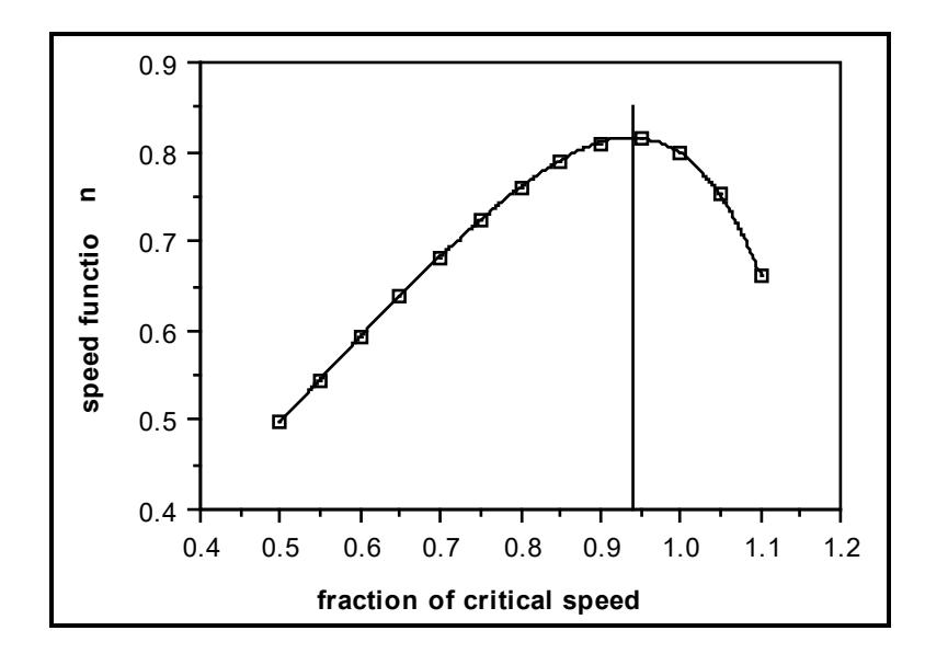
Of particular interest in equation 2.18 is the diameter exponent of 2.3 which Bond changed from an initial value of 2.4. Bond argued that the theoretical exponent was D2.5. This was based on the grinding media mass, at constant volume fraction, varying as D2.0. At constant fraction of critical speed the peripheral speed varied as D0.5 and hence power varied as D2.5. The difference between the theoretical value of 2.5 and Bond's empirically derived 2.3, was thought by Bond to be due to energy recovery from balls falling on the 'down-going' side of the mill.
2.2.5 Hogg and Fuerstenau
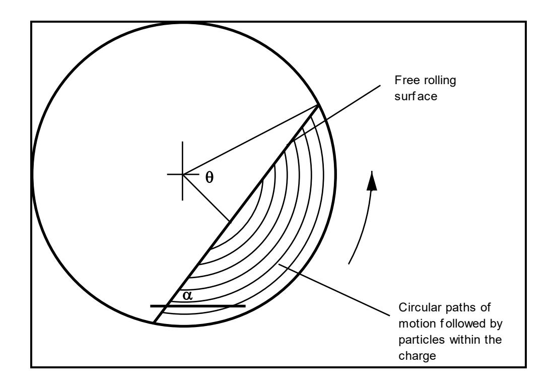
Hogg and Fuerstenau (1972) considered the mill charge to adopt the shape shown in Figure 2.4. In their approach they considered only the rate at which potential energy was gained by particles as they rose up the mill in a locked manner. Once they reach the upper-most point of their upward motion they were assumed to roll down the inclined charge surface and re-enter the charge
lower down. By integrating the rate of potential energy gain over all paths they obtained the following equation:
Power =
$$ K \sin \alpha \sin^3 \theta \phi \rho L D^{2.5} $$
(2.19)
where
\( K = \text{constant} \)
\( \phi = \text{fraction of critical speed} \)
\( L = \text{interior mill length} \)
\( D = \text{interior mill diameter} \)
\( \alpha = \text{charge angle of repose} \)
\( \theta = \text{angle related to mill filling (Figure 2.4)} \)
\( \rho = \text{mean bulk density of the charge.} \)
In deriving this equation the kinetic energy of the charge moving in the locked path was ignored. It was also implicitly assumed that the entire charge was contained within the locked portion. The equation was not applied to industrial mill data.
2.2.6 Arbiter and Harris; Harris, Schnock and Arbiter
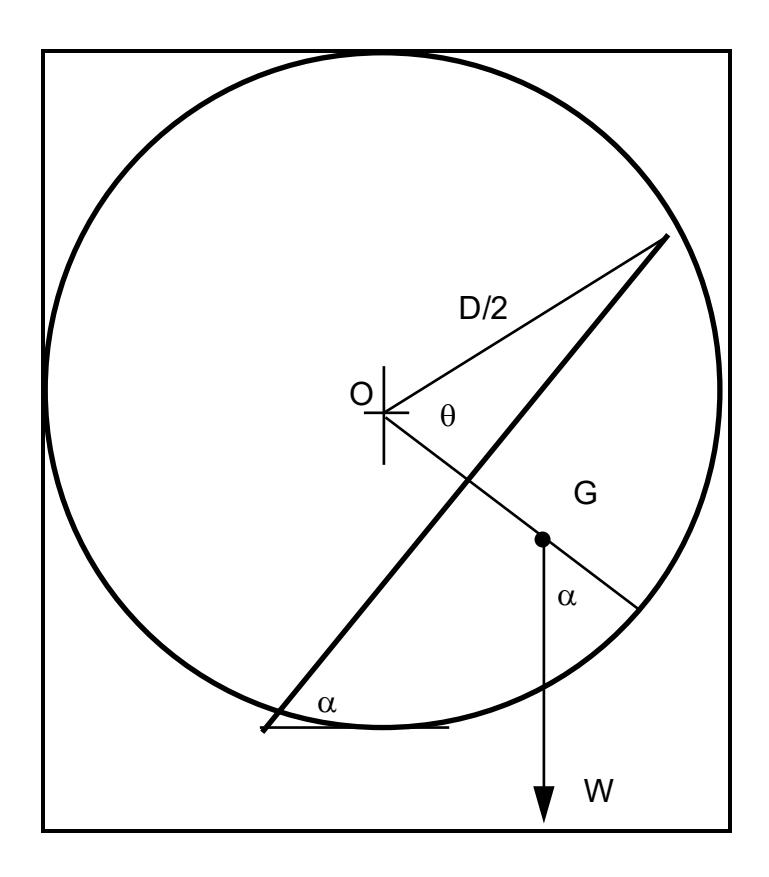
Arbiter and Harris (1982) adopted the same charge shape as Hogg and Fuerstenau but considered power draw from a torque-arm point of view (Figure 2.5).
With reference to Figure 2.5, torque (τ) was defined as:
where
W = mass of charge
OG = torque arm length
The charge mass (W) was given by:
and the torque arm length (OG) was given by:
$$ OG = D \sin^3 \theta / 3\pi L_f $$ (2.22)
where
ρ = charge bulk density
L = mill interior length
D = mill interior diameter.
Lf = load fraction
Using the definition of power (P) as:
where
N = rotational rate
then
$$ P = \frac{\pi \rho g NLD^3 \sin^3 \theta \sin \alpha}{6} $$ (2.24)
This equation is essentially the same as that obtained by Hogg and Fuerstenau (1972).
The term sin3θ was approximated as follows:
$$ \sin^3\theta = 4L_f (1 - L_f) $$ (2.25)
The charge inclination angle (a) was claimed by the authors to have been fitted to the published data of Taggart (1945) and Kjos (1979) from which they determined the values given in Table 2.2. However Harris et al (1985) stated that Kjos reported insufficient operational data and hence it is unclear whether accurate values of a were obtained.
| Type of Mill | a (deg.) |
|---|---|
| Grate | 54 |
| Tube | 48 |
| Autogenous | 45 |
| Overflow | 43 |
| Rod | 34 |
By substituting for sin3θ in equation 2.24, expressing the charge weight as W, and lumping all other terms (including sina), into a constant (k), they simplified their equation as follows:
$$ P = kWND (1-L_f) $$ (2.26)
From the angles given in Table 2.2 values of k were calculated and are shown in Table 2.3.
| Type of Mill | k |
|---|---|
| Grate | 0.13 |
| Tube | 0.12 |
| Autogenous | 0.115 |
| Overflow | 0.11 |
| Rod | 0.09 |
In 1985 Harris, Schnock and Arbiter undertook a very comprehensive review of, essentially, equipment manufacturers' data and power prediction methods. Based on Arbiter and Harris' earlier work they produced a general 'correlation'
equation which could be used to determine the power relationships for different mills and operational conditions. Their equation was presented as:
$$ \frac{P}{D^{2.5} LfY\lambda F (1-aF)} = KD^{n-2.5} $$ (2.27)
or
$$ P = KD^{n}LfY\lambda F (1-aF) $$ (2.28)
where
D = mill diameter
L = mill length
f = fraction of critical speed
λ = charge density
F = fractional filling by the load
K,n,a = parameters
Y = speed correction factor.
Equation 2.28 was used to compare different manufacturers' data and power prediction equations. They concluded from their analysis that substantial differences existed between these equations in their treatment of all the major variables.
It can be inferred from this that little consensus exists between manufacturers as to the effects of the factors that influence mill power draw. This is certainly reflected in the author's experience in assisting mining companies in SAG/AG mill selection. In all cases, for the same mill dimensions and operating conditions, manufacturers' estimates of their power draw varied considerably.
To add to this Harris et al also concluded that considerable errors often exist in measurements of the major variables affecting power. These, they considered, constituted 'the greatest impediment to improving the accuracy of estimating power consumption'.
Their conclusions may be regarded as being critical of both equipment manufacturers and the research community at large, who had not up till that time been able to provide any proven alternative. This was underlined quite clearly in Harris et al's final conclusion which commented on published data availability. They found that, apart from Taggart's offering in 1947, published data were numerous but few were '... complete enough to be useful for power correlation'.
2.2.7 Liddell
Liddell's thesis research (1986), the main conclusions from which were also published in 1988 (Liddell and Moys), appears to be the first comprehensive attempt at experimentally determining the variation in the position and shape of the mill charge under a wide range of speed, filling and slurry rheology conditions, and relating it to power draw. Three of the conclusions from this work were that:
- The maximum power that a mill can draw is a complex function of both speed and filling (see Figure 2.6).
- The models of Hogg and Fuerstenau (1972), Arbiter and Harris (1982) and Bond (1961) did not match well the observed power draw of his 0.545 x 0.305m mill over its full range of speed and filling conditions.
- 'Until the motion of a mill load can be characterized mathematically, the power drawn by the mill cannot be calculated realistically'.
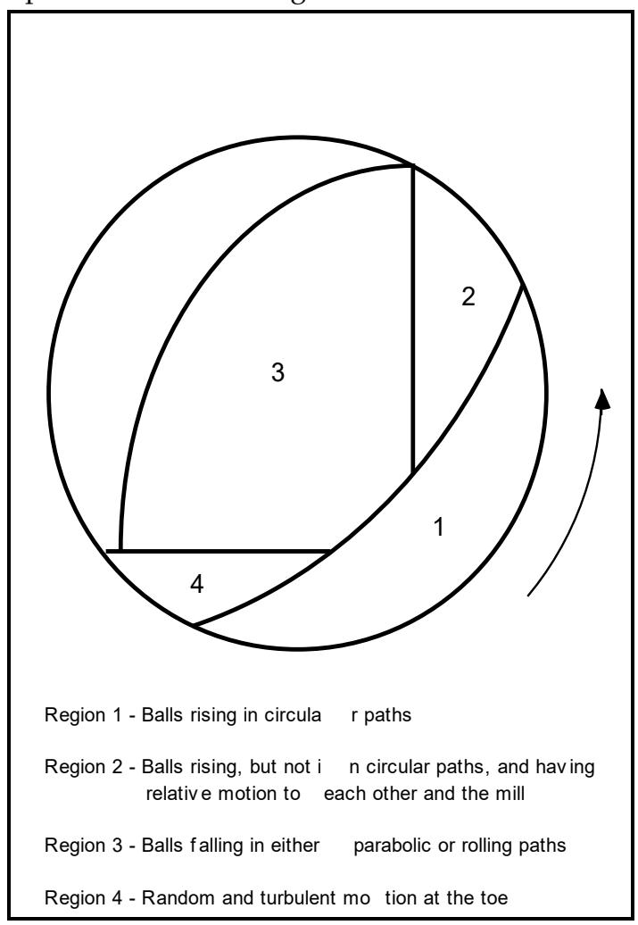
Liddell used high speed cinematographic techniques to view the motion of a mixture of balls and a variety of liquids including water, sand/water and glycerine. For this purpose he used a glass ended laboratory mill. He concluded that the charge could be divided into four regions as shown in Figure 2.7.
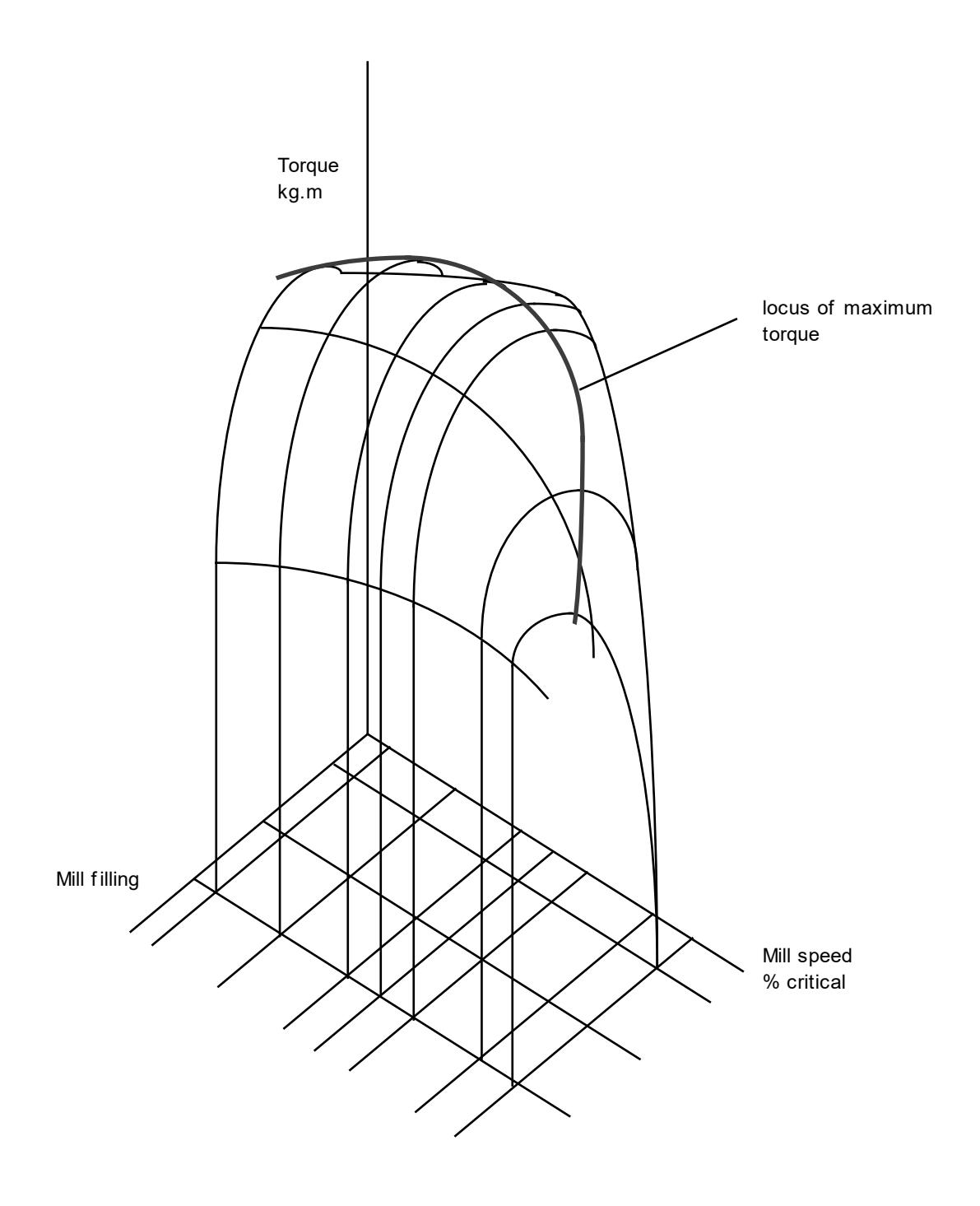
Liddell described the boundaries shown in Figure 2.7 mathematically, making use of Barth's work (1930) in describing an equilibrium surface of logarithmic spiral shape. However, he did not mathematically relate the toe and shoulder position to the mill filling and speed, nor did he attempt to relate his description of the charge to the power draw. Instead he used Harris et al's (1985) correlating equation:
For the filling relationship he used a power maximum at a filling of 0.47. For the speed function (Y) he did not use a specific mathematical relationship but presented tabulated values of the function for a range of speeds. The function was determined from the ratio of the torque at a given speed to the maximum torque. An example of the function is given in Table 2.4.
| Mill Speed (% crit.) | Y |
|---|---|
| 50 | 0.950 |
| 60 | 0.981 |
| 70 | 0.999 |
| 75 | 1.00 |
| 80 | 0.997 |
| 90 | 0.925 |
| 95 | 0.832 |
Liddell argued that his experiments indicated that the speed function varied with different media filling and slurry rheology conditions and that a different Y function was necessary for each of these different conditions. Using Arbiter and Harris' (1982) value for K and a diameter exponent of 2.5, his power equation was given as:
$$ P = 9.69 \rho \phi LD^{2.5} J (1-1.06 J) Y $$ (2.29)
Equation 2.29 fitted Liddell's laboratory mill data well, however he did not apply it to any industrial mill data.
2.2.8 Fuerstenau , Kapur and Velamakanni
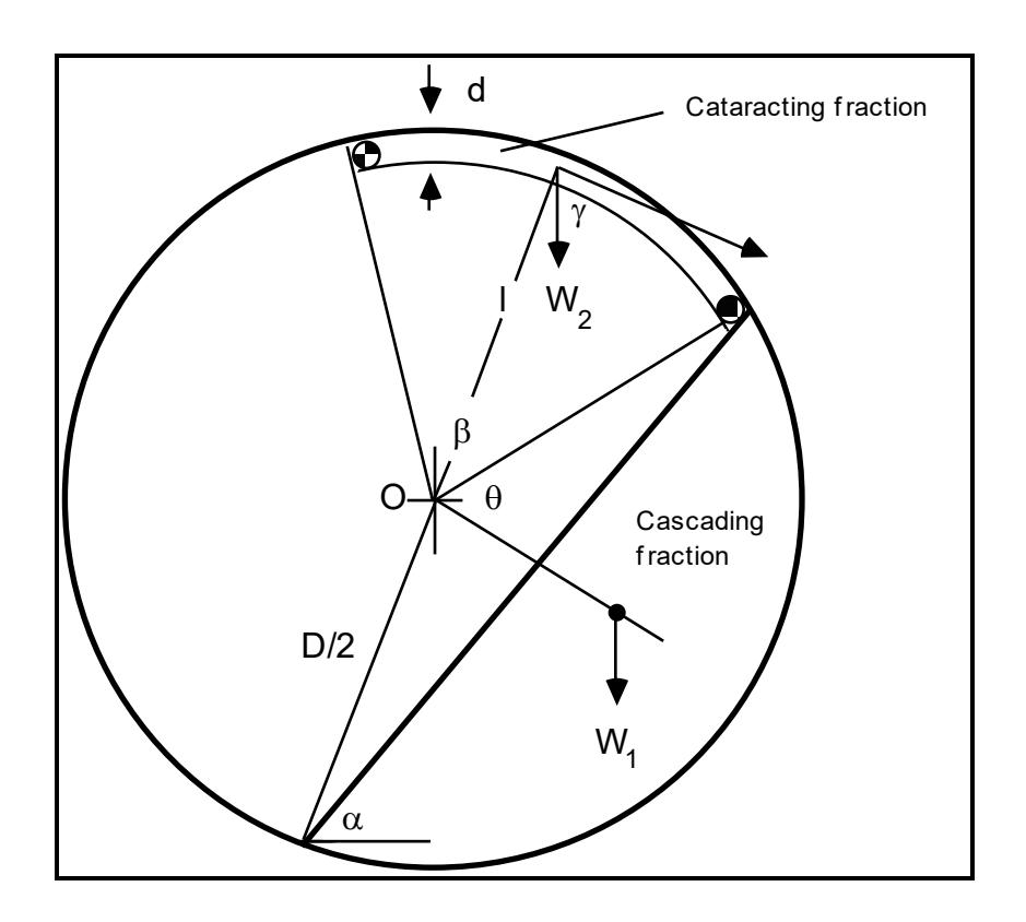
Although Liddell (1986) can arguably be claimed to have been the first to incorporate slurry viscosity in a mill power model, he did so in an implicit and empirical manner via his tabulated speed function. He found that this function varied with media and slurry conditions, notably viscosity. Fuerstenau et al (1990), however, incorporated slurry viscosity in their model in an explicit manner by dividing the charge up into a cataracting fraction which was strongly influenced by the slurry viscosity, and a cascading fraction which wasn't (Figure 2.8).
They divided the weight of the total charge into two fractions using the following equations:
$$ W_1 = (1-E)W $$ (2.30)
W2 = EW(2.31)
where
W1 = weight of cascading charge W2 = weight of cataracting charge
W = total weight of charge
E = parameter.
Similarly the proportion of mill volume that each of the charge fractions occupied was given by:
$$ J_1 = (1-E) J $$ (2.32)
where
J1 = fractional mill filling of cascading charge
J2 = fractional mill filling of cataracting charge
J = fractional mill filling of total charge.
The parameter E was given by the expression
where
z = lumped parameter
x = material related parameter
t = grinding time
t0 = threshold time at which viscosity begins to rise.
The power associated with the cascading charge (Pcs) and the cataracting charge (Pct), were considered separately, in addition to a third power component (Pf) which was related to internal frictional effects. Their general model was stated in terms of the power at a given grinding time t due to their interest in the influence of grind size (which is related to grinding time) on apparent slurry viscosity and power:
$$ P(t) = P_{cs}(t) + P_{ct}(t) + P_{f}(t) $$ (2.35)
where
P(t) = total power draw at grinding time t.
For the cascading power the model of Hogg and Fuerstenau was used in the following form:
$$ P_{cs} = \frac{2NW_1 g (D-d)}{3J_1} \phi(J_1) \sin \alpha $$ (2.36)
where
Ν rotational rate D = mill diameter d = ball diameter
gravitational constant g
\( \phi(J_1) \) \( = 4J_1 (1-J_1); \) \( 0.35 \le J_1 < 0.5 \) 4J1 (1.05 - 1.33J1); \( 0.2 \le J_1 < 0.35 \) .
For the power of the cataracting fraction they used the following equation:
where
γ
1 = lever-arm length \( \approx 0.5(D-d) \) = \( \alpha \) + \( \theta \) + \( \beta \) /2 - 90 (see Figure 2.8).
The angle \( \beta \) was given by the expression:
$$ \beta = \frac{E\pi}{2\psi(d)} \left[ 1 - \frac{\psi(d)}{D} \right]^{-1} $$ (2.38)
where
function (unspecified) of ball size. \( \psi(d) \)
The friction power was given as:
where C, k are constants.
The model contained six parameters which required to be fitted, though as \( \psi(d) \) was unspecified, it too, presumably, would also require fitting. Its usefulness in most practical situations where limited data are available, must therefore be considered to be limited.
2.2.9 Moys
Moys' paper (1990), like Fuerstenau et al's (1990), also reflects an interest in viscosity effects on power draw, in addition to those of liner design and mill speed. His conceptual model was, in some ways, similar to Fuerstenau et al's in that it also partitioned the mill charge into two fractions. One part was described as a non-centrifuging portion whose power draw, like Fuerstenau et al's cascading fraction, could be described by a simple torque-arm approach. The other portion centrifuged and drew no power. This provided a simple but effective way of incorporating the effect on power draw of changes in speed, liner design and viscosity, by relating them to the thickness of the centrifuging layer. Thus as the centrifuging layer increased the tendency would be to reduce the mill power draw.
Moys chose to use Bond's equation for the non-centrifuging fraction, though without Bond's speed correction factor. To use the equation the effective filling of the non-centrifuging fraction (Jeff) was required to be calculated. This was done using the following equation:
$$ J_{\text{eff}} = \frac{J - 4 \delta_{c} (1 - \delta_{c})}{(1 - 2\delta_{c})^{2}} $$ (2.39)
where
δc = thickness of the centrifuging layer
J = total fractional mill filling.
A simplified form of Equation 2.39 was also given for J = 0.5 and small values of δc:
The power equation for the non-centrifuging charge was given as:
$$ P = K_2 D_{eff}^{2.3} \sin \alpha \rho_L J_{eff} (1 - \beta J_{eff}) N_{eff} $$ (2.41)
where
Deff = (1 - 2δc) D
a = angle of repose
ρL = bulk density of the load
Neff = undefined - though was presumably the fraction
of critical speed at D = Deff
β = parameter K2 = constant.
To describe the centrifuging layer thickness (δc) Moys proposed the following empirical formula:
$$ \delta_{c} = J^{\Delta J} e^{-\frac{N_{100} - N}{\Delta N}} $$ (2.42)
where
∆J, N100, ∆N = parameters.
Using data from a 0.53 x 0.3m laboratory mill, fitted with four different lifter designs/configurations, Moys fitted his model parameters using both equations 2.39 and 2.40. He concluded that the simplification of using equation 2.40 did not have a significant effect on the model's ability to describe his power data. Some of the model parameters were found to be related to liner design but further research was deemed necessary. The model was not applied to any full scale mill data nor was it applied to power data relating to slurry viscosity effects. Its structure, however, lends itself to empirical modelling of such effects by adjusting the values of the parameters in equation 2.42.
2.2.10 Austin
From his literature search, Austin (1990) concluded that for semi-autogenous mills there were 'no generally accepted mill power equations comparable to those of Bond'. He therefore used elements of Hogg and Fuerstenau's equation (1972) and Bond's (1962), plus some additional modifications, to provide a model which was claimed to be suitable for SAG mills with both high and low aspect ratios.
He firstly took Hogg and Fuerstenau's equation as follows:
$$ M_{p} = K \sin \alpha \sin^{3}\theta \phi_{c} \rho_{c} LD^{2.5} $$ (2.42)
where
Mp = net mill power
a = angle of repose
θ = angle related to mill filling (Figure 2.4)
ρc = mean charge density
φc = fraction of critical speed
K = constant.
It is implicitly assumed in this equation that the energy input to the mill is required to lift the charge in a locked manner until it reaches the upper part of the slip surface. The potential energy it has at this point is subsequently entirely consumed as it moves to the lower part of the slip surface where it re-enters the locked charge. The equation therefore neglects the energy which the mill must input to provide the kinetic energy of the particles moving in the locked charge. Austin therefore modified equation 2.42 as follows:
$$ M_{p} = K \sin\alpha \sin^{3}\theta \phi_{c} \rho_{c} LD^{2.5} (1 + \gamma) $$ (2.42)
where
γ = kinetic energy fraction of the net power
He found that for most practical situations \( \gamma \) varied in the range 0.22 - 0.30 and therefore was incorporated in the constant (K).
For \( \sin^3\theta \) the following approximate relationship for J in the range 0.2 < J < 0.5 was used:
where
J = fractional volume of the cylindrical section of the mill filled by total charge.
For the mean charge density \( (\rho_c) \) he used the following expression:
$$ \rho_{c} = (1 - E_{B}) J (\rho_{s}/w_{c}) + 0.6J_{B} (\rho_{b} - \rho_{s}/w_{c}) $$ (2.44)
where
\( E_B \) = effective porosity of the bed of rocks and balls = 0.3
\( w_c \) = weight fraction of rock to water and rock in the
mill charge \( \approx 0.8 \)
ρb = density of ball material
\( \rho_{\rm S} \) = mean density of rock
JB = fractional volume of the cylindrical section of the
mill filled by balls only.
To allow for the reduction in mill power observed when the speed of the mill exceeds a certain critical value, he used Bond's empirical speed correction factor \( (f(\phi)) \) :
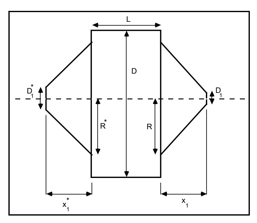
For high aspect ratio mills, i.e. a high ratio of D/L, it is often found that conical ends are incorporated in their design. Austin developed an equation for predicting the power draw of the conical ends by considering the power draw of the elements shown in Figure 2.9 and integrating with respect to the filled length of the cone.
With reference to Figure 2.9 the fraction of the total power attributed to the conical ends \( (f_3) \) was given as:
$$ f_{3} = \frac{0.046}{J(1-AJ)} \left\{ \left( \frac{x_{1}/L}{1-D_{1}/2R} \right) \left[ \left( \frac{1.25 R/D}{0.5-J} \right)^{0.1} - \left( \frac{0.5 - J}{1.25 R/D} \right)^{4} \right] + \left( \frac{x_{1}^{*}/L}{1-D_{1}^{*}/2R^{*}} \right) \left[ \left( \frac{1.25R/D}{0.5 - J} \right)^{0.1} - \left( \frac{0.5 - J}{1.25 R^{*}/D} \right)^{4} \right] \right\} $$ $$ (2.46) $$
His final equation for the mill power draw was therefore given as:
$$ M_{p} = KD^{2.5} L(1 - 1.03J) \left[ (1-E_{B}) (\rho_{s}/w_{c}) J + 0.6J_{B} (\rho_{b}-\rho_{s}/w_{c}) \right] $$ $$ \phi_{c} \left[ 1 - \frac{0.1}{2^{9-10\phi_{c}}} \right] (1 + f_{3}) $$ (2.47)
where
K = lumped constant including the term sinα.
Austin used data from a high aspect ratio mill (Tanaka and Tanaka, 1983) and a low aspect ratio mill (Flook and Bailey, 1979) to determine a value for K. The resultant value suggested by Austin was K = 10.6.
2.2.11 Mishra and Rajamani
The rapid development of high powered yet cheap computers has considerably stimulated the field of mathematic modelling and simulation in recent years (McKee and Napier-Munn, 1990). In particular the application of discrete element methods (DEM) is becoming more prevalent. The methodology was pioneered by Cundall and Strack (1979) originally in the field of soil mechanics. However it is inherently suited to the analysis of particulate systems. It hence has enormous potential in the field of mineral processing and has been used to describe jig bed motion (Beck, Jonkers and Holtham, 1993) and ball mill simulation (Mishra and Rajamani, 1990).
Currently most implementations of DEM are two-dimensional and hence the particles in question are reduced to discs. The DEM algorithm identifies each disc individually and keeps a record of its relevant properties including position and velocity. This record is updated every incremental time step. When two discs overlap, ie. a contact occurs, the resultant forces are computed. The forces are modelled using a pair of normal and tangential spring dashpots, the latter having the facility for friction damping effects.
Providing the physical properties of the material and the forces acting on a single body are properly described, DEM should theoretically describe in minute detail the motion, and hence energy, of all the particles within a system.
Mishra and Rajamani (1990) modified existing DEM code (Corkum, 1989; Cundall and Strack, 1979) for application to ball mills and added (among other things) the ability to calculate the mill torque. This was done by assuming that the mill torque can be calculated from the shear forces acting on the wear face of the liners.
Thus the net torque (T) was given by:
$$ T = \sum_{i=1}^{n} r_i \times F_{\text{shear, i}} $$ (2.47)
where
ri = position vector of disc i in contact with the mill
Fshear,i = shear force acting at the contact.
To verify their approach with respect to the prediction of mill power draw, they simulated the mill used by Liddell and Moys (1989) and found good agreement. This result augers well for further development of this technique. Despite the rapid developments in computer hardware, a severe limitation is still the time taken for DEM computer code to execute - Mishra and Rajamani quote the requirement of 7.84 hours of CPU time on an IBM 3090 super computer to run a simulation of the Liddell and Moys mill, with 148 balls contained in it running at 40% of critical speed.
2.3 CONCLUSIONS
In the almost 100 years that have so far passed in this century no publication has been found which presents an equation, or series of equations (model), with convincing attendant evidence of its ability to accurately predict the power draw of a wide range of industrial grinding mills under a wide range of operating conditions. This lack of relevant experimental data has consequently limited the practical application of many of the attempts at modelling mill power draw. Data on the power draw of grinding mills in the literature do abound, but as Harris et al (1985) remarked they are "... too frequently unusable simply because one or more essential variables have been omitted". The absence of published results from vigorous experimental testing of the various models has resulted in a general lack of evaluation of the validity of assumptions and hypotheses that such models contain. Harris et al (1985) however, did make some efforts in attempting to evaluate the performance of various power prediction equations and in so doing further developed a semi-empirical one of their own. However, in using manufacturers' published data, which themselves were undoubtedly generated by proprietary equations of unproven validity, they most likely succeeded in generating little more than a concensus of the various errors in these models.
Liddell's work (1986) in particular, clearly highlighted the deficiencies of a number of the more popular mill power equations. He showed that in the case of his laboratory mill, none of these equations was able to predict its power draw over a wide range of speeds.
This literature review has concentrated on the more important research developments in the field of mill power modelling and in so doing reviewed 11 pieces of published work. What transpires from this review is that, in terms of the core structure of the equations they contain, there is little to chose between most of them. As a result the form, if not the exact parameter values, of the semiempirical equation of Bond is seen repeated in all subsequent work, with the exception of Mishra and Rajamani (1990). Their work, and that of Cundall and Strack (1979) whose DEM code they modified, should be applauded in that it represents a truly original approach to the modelling of mill power draw. The enormous amount of computing time that their method needs, however, is likely to see its practical application limited for some time to come.
There is no doubt from this literature review, and from the conclusions drawn from similar exercises by such researchers as Harris et al (1985), that there does not exist a published source of good quality, wide ranging industrial data from which an accurate power model can be developed. It is also equally clear that there does not exist a model of proven accuracy which can be used to predict the power draw of ball, SAG and AG mills under the full range of operating and design conditions in which they are found in industry.
CHAPTER 3
CHARGE MOTION IN WET TUMBLING MILLS
From the literature review in Chapter 2 it is apparent that a major limitation of most published mill power models is that they lack any explicit description of the motion of the charge and the way that it varies with speed and filling. In this chapter a photographic technique to examine charge motion is described. The results from experiments using this technique are presented, together with equations which describe both the changes in charge shape and velocity that were observed as the mill filling and speed were varied.
3.1 INTRODUCTION
The rotation of a cylindrical tumbling mill moves the charge it contains and in so doing consumes energy. The key to determining the rate at which this energy is consumed (power) is in being able to describe the motion of the charge. Taggart's comments (1945) in this regard are particularly relevant: 'Net power is not capable of analytic determination because of present ignorance of the internal dynamics of the tumbling load'. This chapter describes the results of experiments designed to provide such information. The results are subsequently used in the development of a mill power model.
3.2 EXPERIMENTAL DETAILS
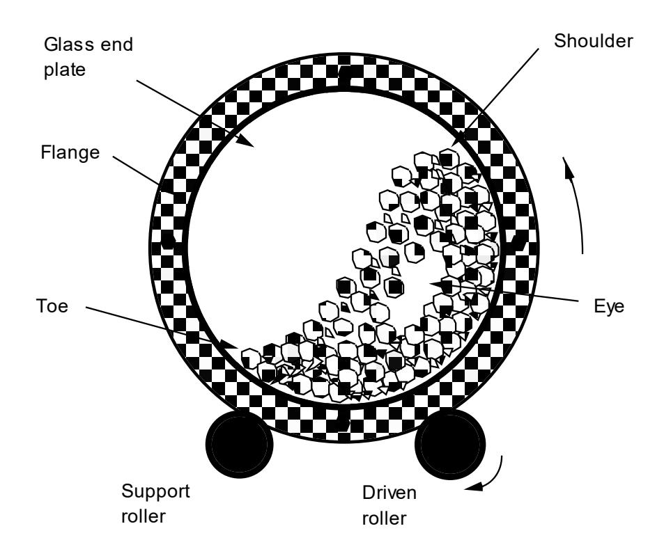
The main aim of the experimental stage was to determine how the shape of the mill charge changed as both the volume of the charge and rotational speed were varied. A laboratory tumbling mill was used for this purpose. It comprised a 300 x 150mm (D x L) glass fronted mill mounted on two rollers (Figure 3.1). A motor and variable speed controller were coupled to one of the rollers enabling the mill to be rotated in the range 73 - 112% of critical speed. A rock charge was used in the mill, the size distribution of which was a scaled version of an equilibrium charge obtained during a 6' x 2' fully autogenous pilot mill test. The size distribution of the charge is shown in Table 3.1. A nickel sulphide ore was chosen for the charge due to its uniform colour. The charge was prepared by crushing relatively large lumps in a jaw crusher and sizing them on a 2 sieve series. The required amounts from each size fraction were then combined to produce the distribution shown in Table 3.1. The charge was subsequently tumbled to ensure that the particles were rounded in shape. The charge was then removed, washed, dried, re-sieved and the amounts in each size fraction adjusted to correspond to that given in Table 3.1.
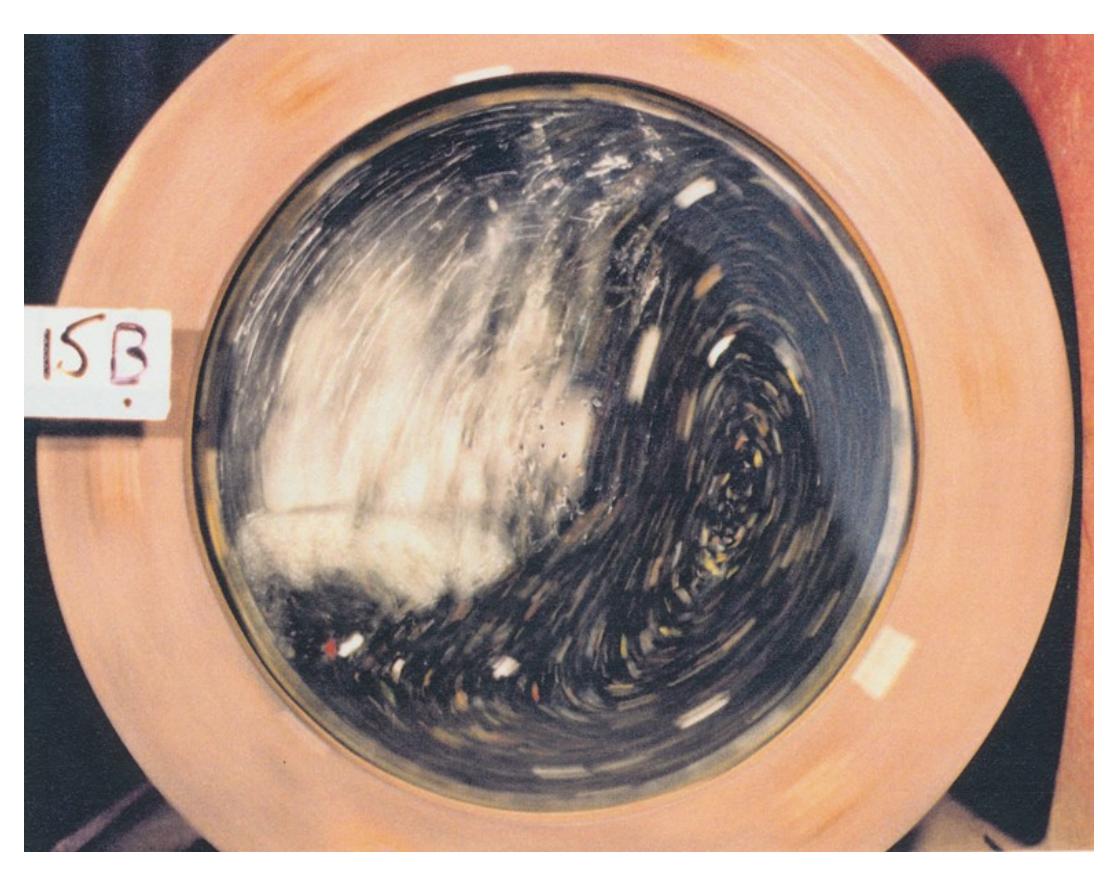
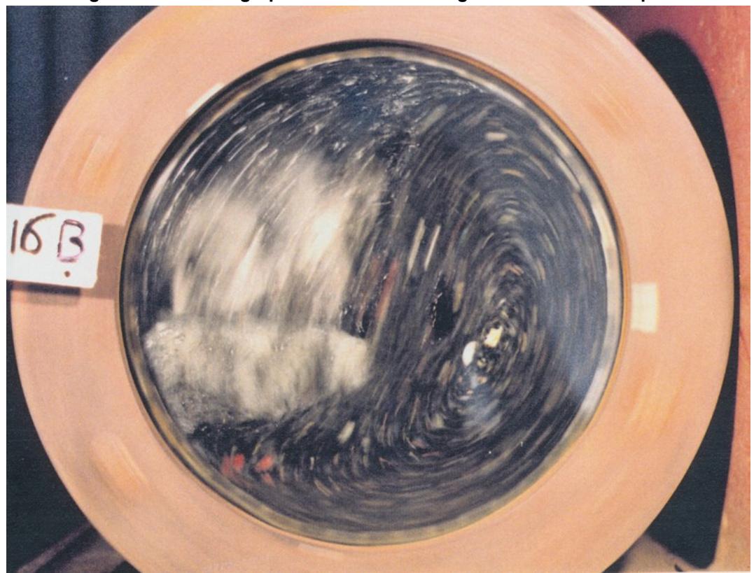
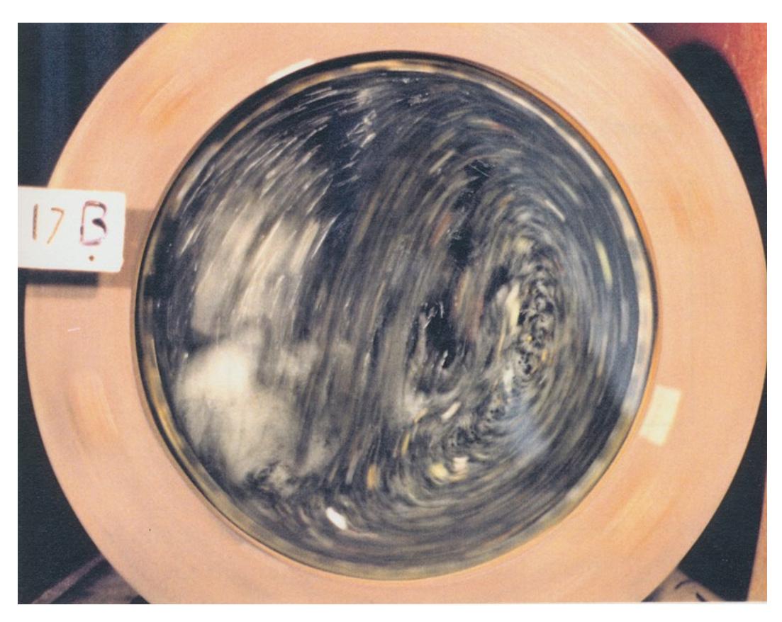
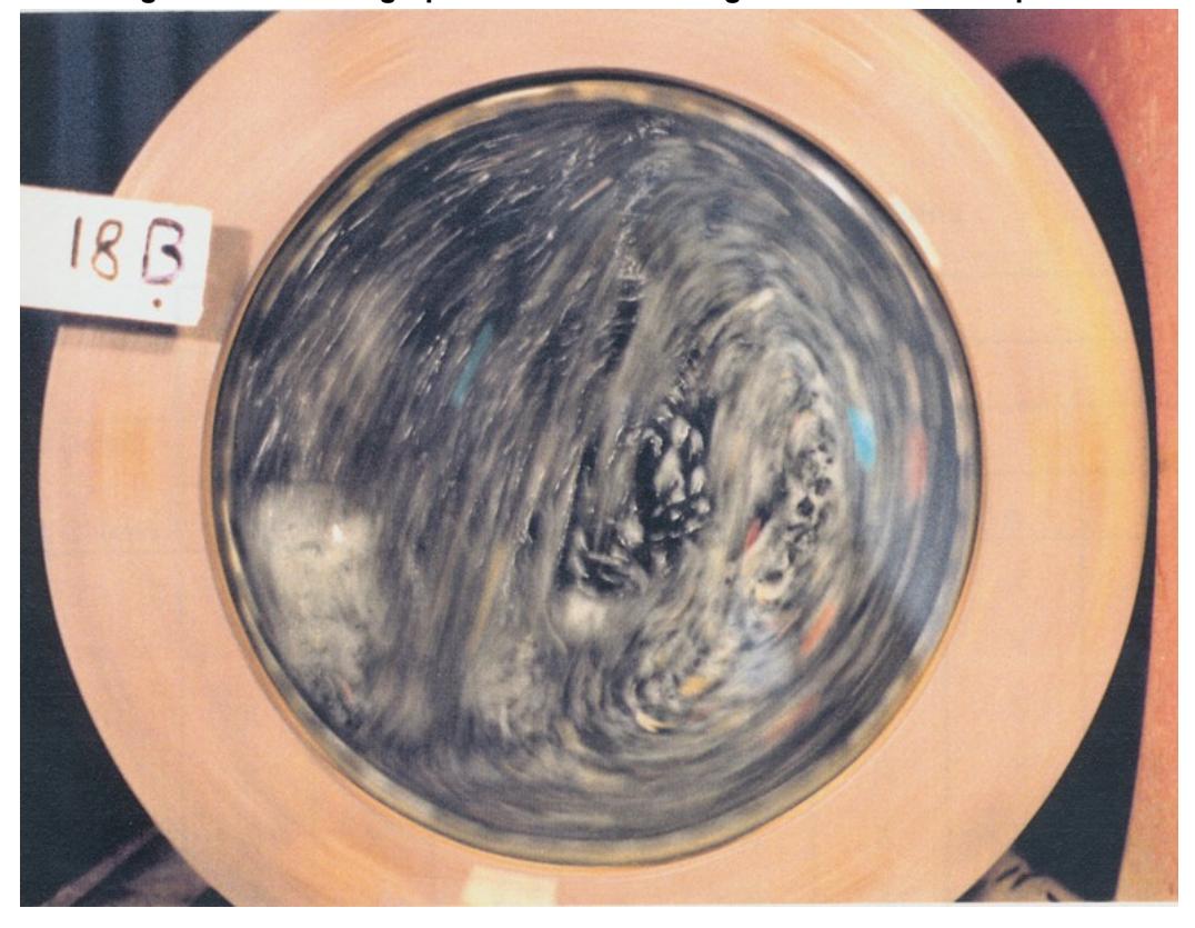
A photographic technique was employed to provide a source from which measurements of the charge shape and velocity could be made. Brightly coloured tracers, made by painting a number of the rocks in bright colours, were added to the mill charge. Once the mill was set in motion still photographs of the charge were taken through the glass end using a very slow shutter speed. As the mill charge was a uniformly dark nickel ore, the tracers were clearly visible in the photographs as lines of colour. Apart from highlighting the general shape of the charge, the length of each line provided information on the speed of individual particles at different locations within the charge. A velocity field description of the charge was thus able to be built up. Examples of the resultant photographs are shown in Figures 3.2a - 3.2d for a 45% mill filling at speeds of 73%, 78%, 86% and 95% of critical. The method thus provided a two dimensional picture of the mill charge rotating against the glass end plate. It was assumed that end effects were negligible and that no segregation occurred along the length of the mill.
| mm | % retained |
|---|---|
| 16 | 0 |
| 11.2 | 3.6 |
| 8.0 | 34.2 |
| 5.6 | 25.7 |
| 4.0 | 16.3 |
| 2.8 | 5.2 |
| 2.0 | 6.1 |
| 1.0 | 8.9 |
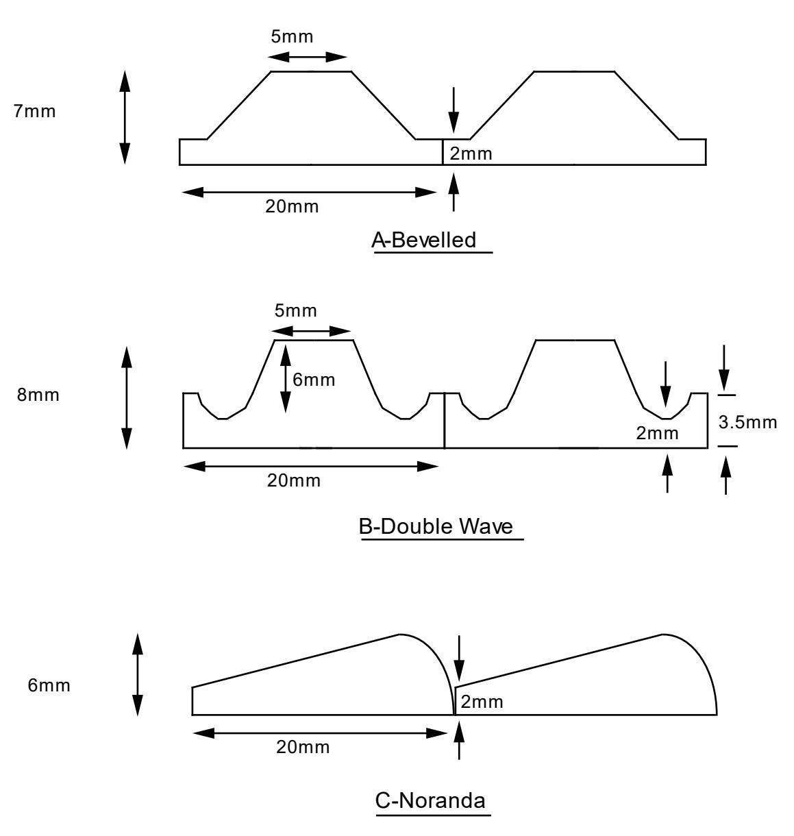
Details of the full range of experimental conditions covered are given in Table 3.2. Over this range of mill loads and speeds, 3 different lifter types were used, the details of which are shown in Figure 3.3. Their choice was dictated by the need to determine the extent to which the charge pattern, and by inference - the power draw, would change with gross changes to their design.
| Mill Filling (%) | |||||||||
|---|---|---|---|---|---|---|---|---|---|
| 15 | 30 | 45 | |||||||
| Speed | Lifter Type | ||||||||
| (% Critical) | A | B | C | A | B | C | A | B | C |
| 73 | X | X | X | X | X | X | X | X | X |
| 78 | X | X | X | X | X | X | X | X | X |
| 86 | X | X | X | X | X | X | X | X | X |
| 95 | X | X | X | X | X | X | X | X | X |
| 102 | X | X | X | X | X | X | X | X | X |
| 112 | X | X | X | X | X | X | X | X | X |
3.3 VARIATION IN TOE AND SHOULDER POSITION
3.3.1 Measurement Details
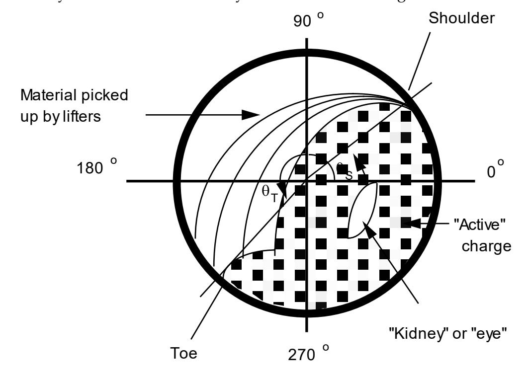
From the photographs of the laboratory mill, the general pattern of the charge that was observed is as shown schematically in Figure 3.4. As the mill rotates the charge is lifted up the rising face of the mill until the shoulder is reach. At this point the bulk of the charge falls away towards the toe region. In addition small amounts of material are discharged as a 'spray' which in some cases impact directly onto the exposed liners on the opposite face of the mill.
Measurements from the photographs were made of the angular displacement of the toe and shoulder. A pictorial definition of these measurements together with relevant symbols and co-ordinate system can be seen in Figure 3.4.
Duplicate tests of the measurement of the shoulder and toe position were conducted to determine experimental error. The resultant 95% confidence interval for measurement of the shoulder angle ( \( \theta_S \) ) was found to be \( \pm 6.5 \) degrees, whilst that for the toe angle ( \( \theta_T \) ) was found to be \( \pm 4.8 \) degrees.
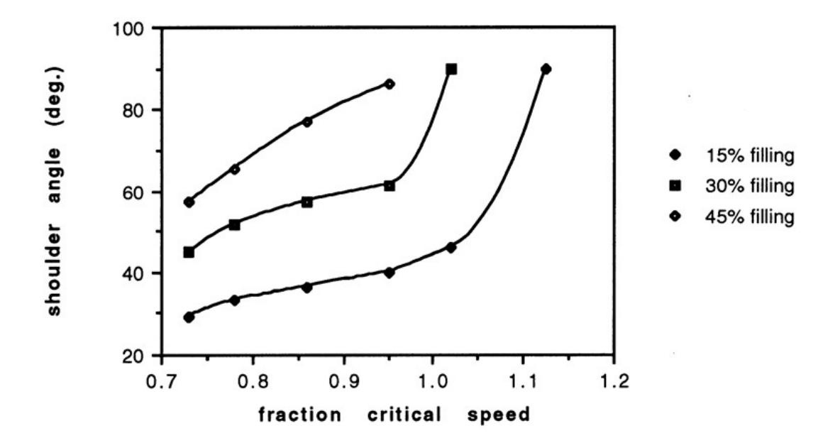
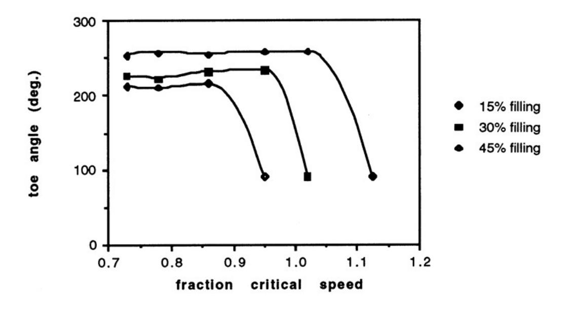
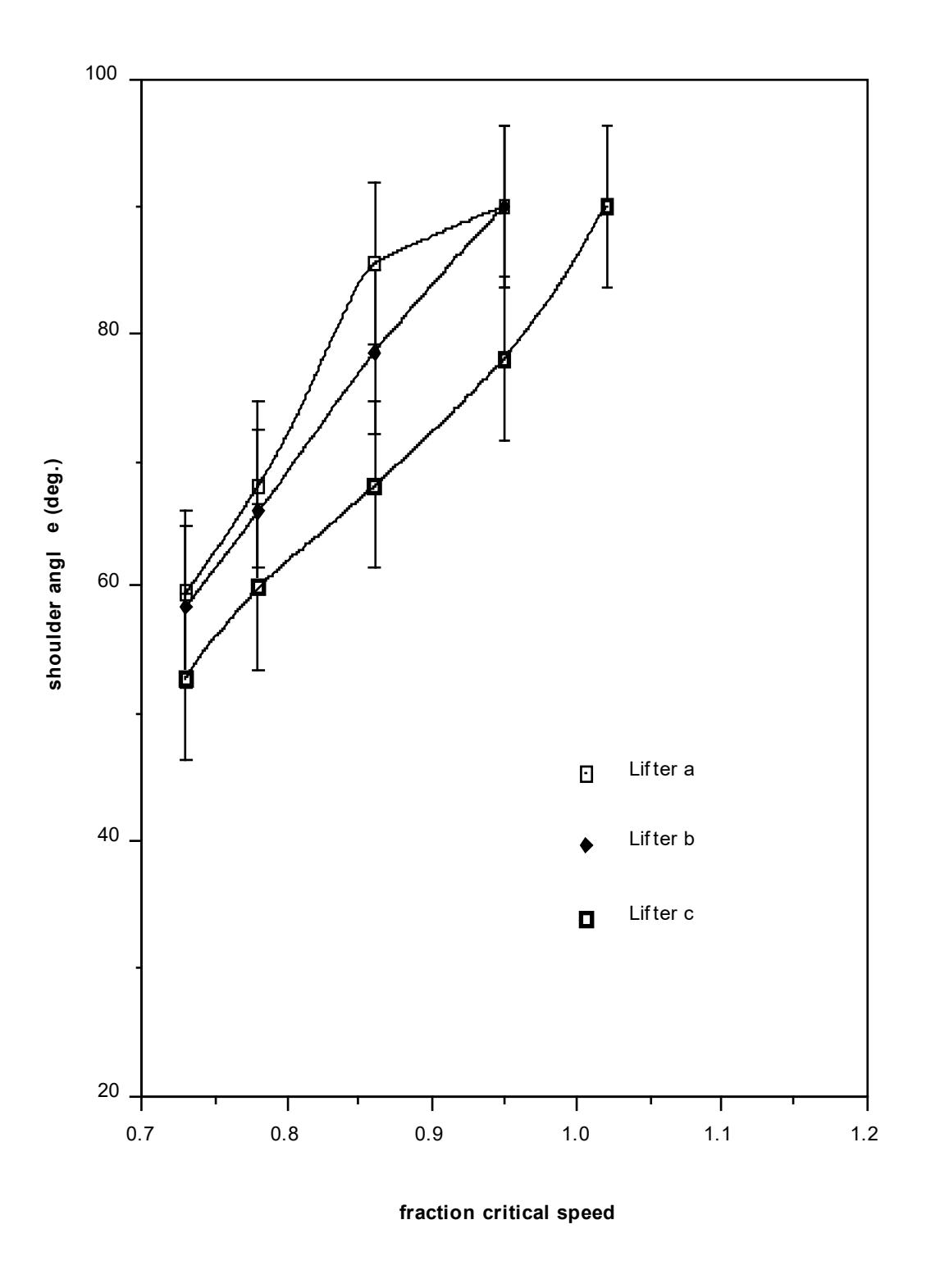
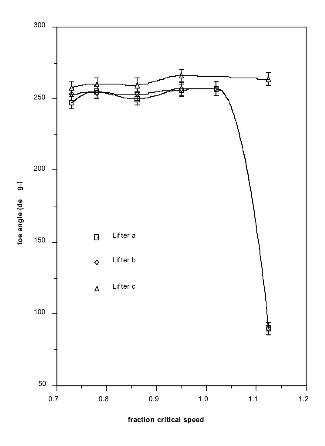
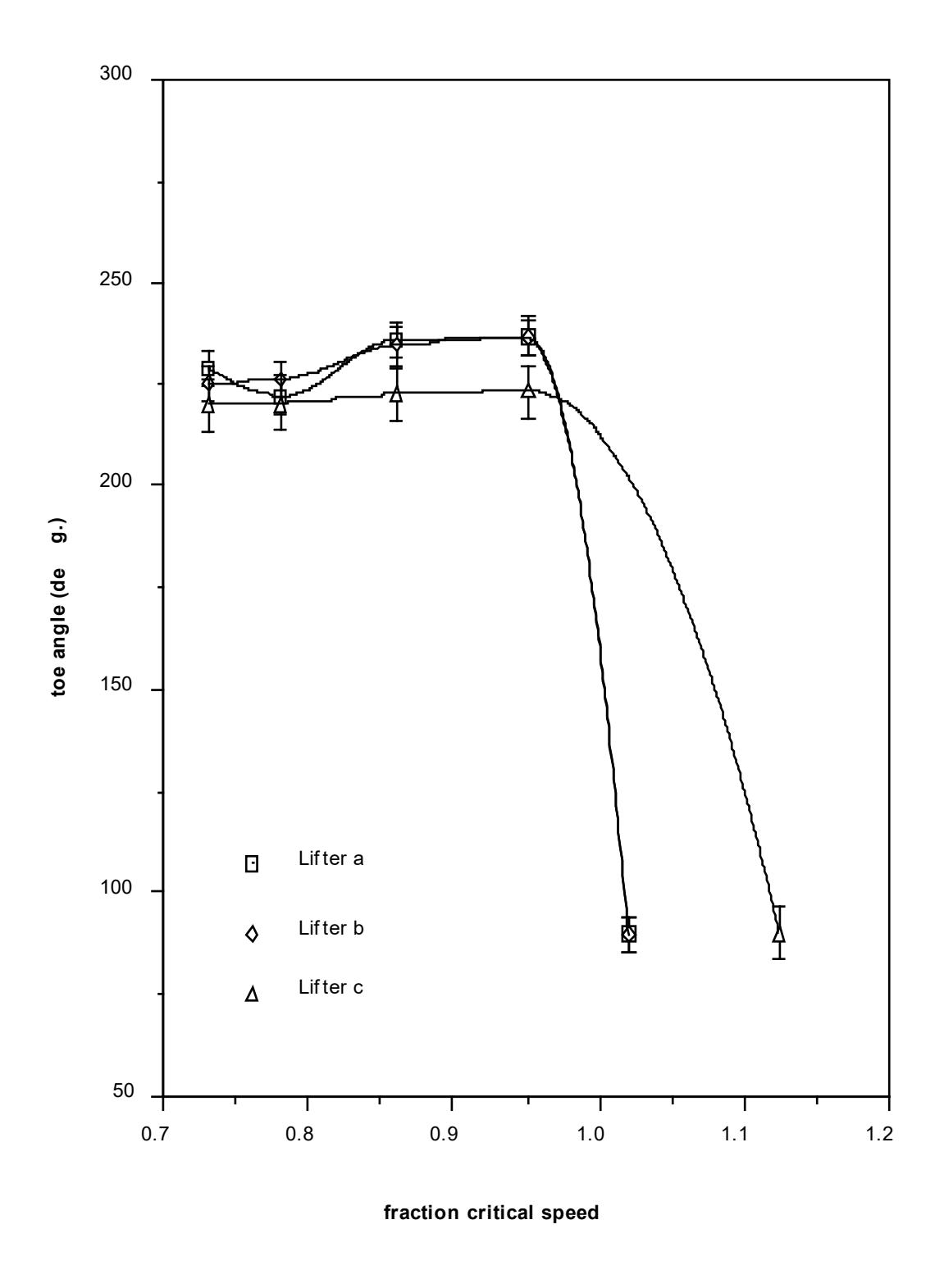
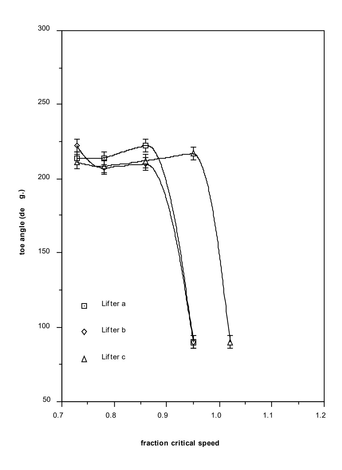
Details of the measurements are given in Appendix 1 for each of the 3 lifter types used. Mean values were also calculated and are given in Table 3.3. These data are plotted in Figures 3.5 and 3.6 to illustrate the variation in toe and shoulder position with mill filling and speed.
| Mill Filling (%) | ||||||
|---|---|---|---|---|---|---|
| Speed | 15 | 30 | 45 | |||
| (% Critical) | ΘS | ΘΤ | ΘS | ΘΤ | ΘS | ΘΤ |
| 73 | 31.3 | 252.7 | 45.0 | 225.0 | 57.3 | 213.0 |
| 78 | 33.0 | 256.3 | 51.7 | 223.0 | 64.7 | 210.3 |
| 86 | 36.7 | 254.0 | 57.7 | 231.3 | 77.7 | 215.0 |
| 95 | 45.0 | 259.7 | 62.0 | 234.3 | * | * |
| 102 | * | * | * | * | 90 | 90 |
| 112.5 | 90 | 90 | 90 | 90 | 90 | 90 |
Note: * indicates the onset of centrifuging.
3.3.2 Effect of Speed
The effect of increasing mill speed is to raise the charge higher and hence increase the shoulder angle (Figure 3.5). After leaving the mill shell at the shoulder, the charge falls to the toe region where it tends to 'pile-up' whilst waiting for the mill to accelerate it to its rotational velocity. The toe position, as a result, appears not to vary over most of the speed range for a given mill filling. Eventually a speed is reached where centrifuging begins. At this point the shoulder and, in particular, the toe angles rapidly tend to the 90° position. The entire charge does not centrifuge at the same speed, however. The outer layers centrifuge first. Further increases in speed cause more and more layers to centrifuge until eventually the entire charge is centrifuging. Once centrifuging commences measurements of the shoulder and toe position of the remaining charge becomes increasingly difficult. The speed at which centrifuging commenced and at which the majority of the charge centrifuged were measured, however.
3.3.3 Effect of Mill Filling
The mill filling is also seen to influence the toe and shoulder position. Larger mill fillings give rise to higher shoulder angles but lower toe angles. As a result, the mill speed at which centrifuging commences is seen to be a strong function of the mill filling, with higher fillings centrifuging at much lower speeds. This effect is a departure from the classical view of a single centrifuging speed dictated solely by the balance of gravitational and centrifugal forces. In such an approach interaction effects are ignored. However, it is clear that the charge behaves as a collective body and that interactions cannot be ignored. Thus, within the charge the material lower down the rising face of the mill pushes the higher material further than would be the case with single particles moving inside the mill. With higher mill fillings this pushing effect is more pronounced and gives rise to higher shoulder angles. The height to which the charge is lifted is related to mill speed and the magnitude of the frictional forces within the charge. These in turn are dictated by the charge weight. The relative magnitude of these are independent of mill diameter. Hence the relative position of the charge will be the same regardless of mill diameter providing the mill filling and the % of critical speed remains constant.
3.3.4 Effect of Lifter Type
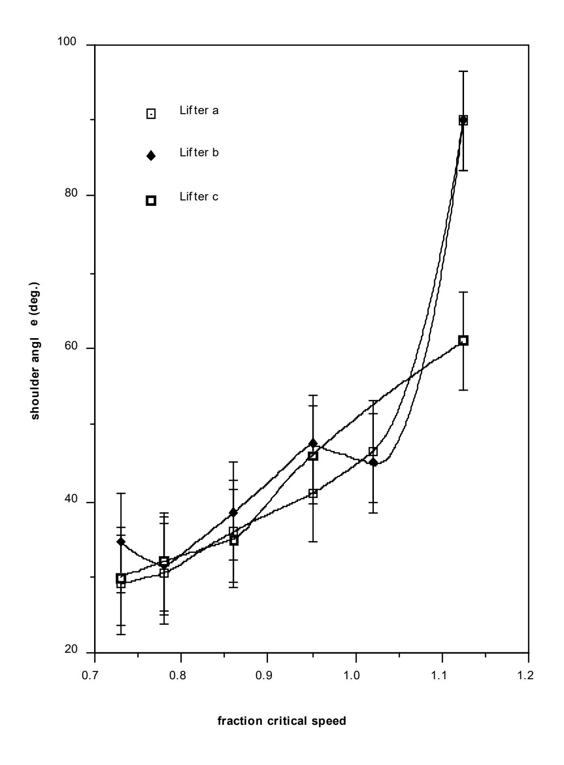
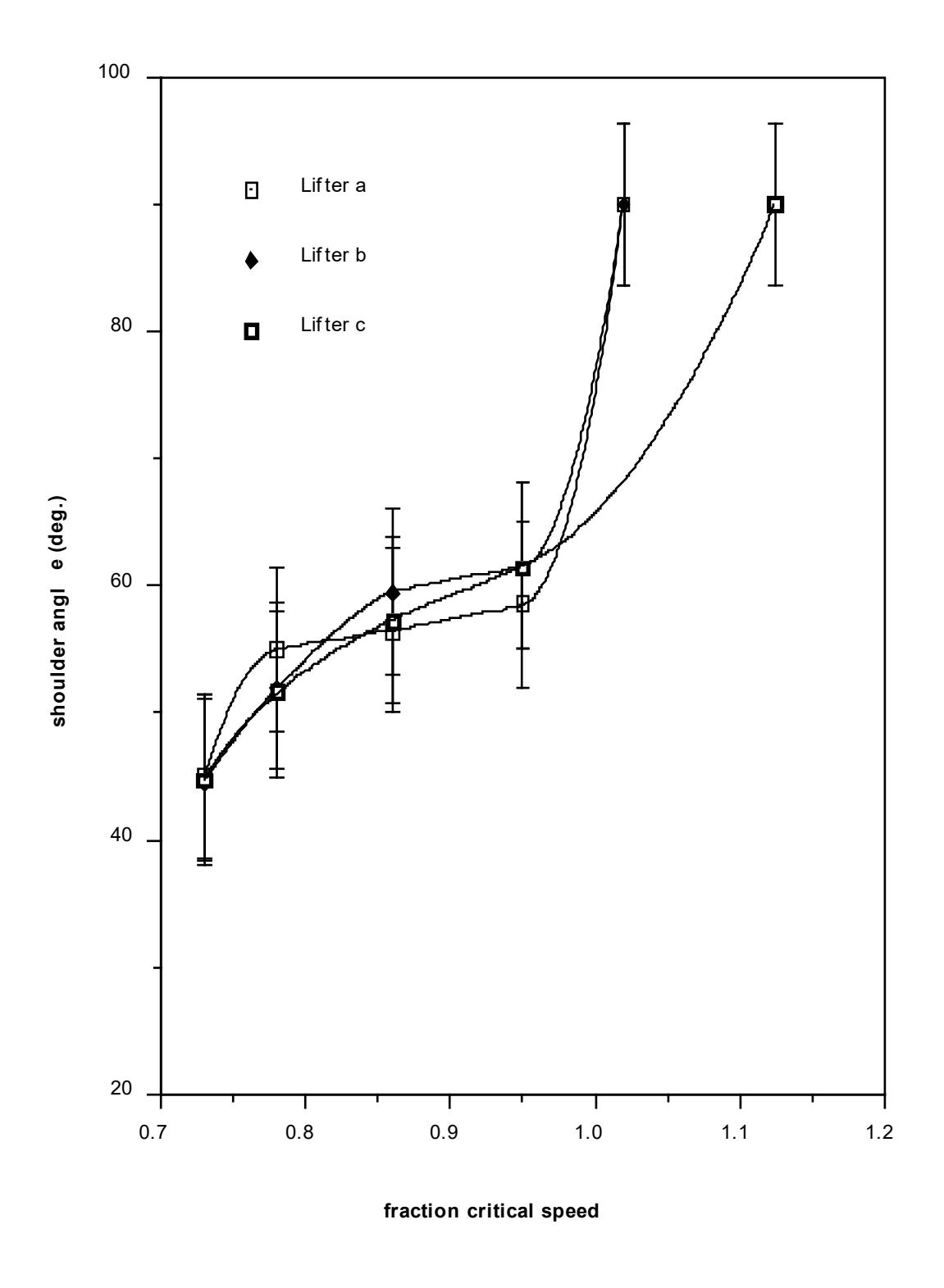
A description of the 3 lifter types used was given in Section 3.2. The lifter types were scaled versions based on those used in a 7.2m diameter SAG mill. The measurements made of the toe and shoulder positions for each lifter type are shown graphically in Figures 3.7 - 3.12. Measurement error bars associated with a 95% confidence interval are also shown.
Scatter in the data makes consistent trends difficult to determine. However, in general lifter type B provides a similar lift to type A, both of which lift higher than type C. In consequence the charge centrifuges at the lowest speeds using lifter types A and B, and the highest speeds using type C. Differences between the lifters are not large, however, with variations in the shoulder and toe angles for most of the filling and speed range being within experimental measurement error. Only at very high speeds (i.e. > 95% of critical) or high mill fillings (45% of mill volume) do differences become pronounced. Statistically, therefore, it can be argued that a single relationship could be used to describe the effect of all the lifter types over the range of mill filling and speeds normally found in industrial mills.
3.3.5 Mathematical Description of the Variation in Toe and Shoulder Position
To provide a mathematical description of the variation in angular displacement of the toe and shoulder which would be applicable over a wide range of lifter types, the data from each of the 3 lifters were averaged. The previous section showed this to be a reasonable approach over most of the speed and filling range. The implicit assumption in this approach is that changes to the lifters have a relatively small effect on power draw. This suggestion is supported by the experiments of Rose and Evans (1956) whose results indicated a maximum power draw change of only 5% over a range of lifter heights varying from 0.02 - 0.2 of the diameter of their test mill.
To describe the variation in toe angle the following equation form was used:
$$ \theta_{\rm T} = A(1 - e^{-B} (\phi_{\rm c}^{-\phi})) + \pi/2 $$ (3.1)
where
A, B = functions of the fractional mill filling (Jt).
φc = is the experimentally determined fraction of the theoretical critical speed at which centrifuging was fully established ie. the majority of the charge was centrifuging. It is also a function of Jt of the form C + DJt where C and D are constants.
φ= is the fraction of theoretical critical speed that the mill is run at.
θT = toe angle (rads.).
To ensure that at centrifuging speed the angular displacement of the toe and shoulder converged to the same value (π/2 radians), the shoulder angle (θS) was chosen to be expressed as a function of θT. The following equation form was used:
$$ \theta_{\rm S} = \pi/2 - (\theta_{\rm T} - \pi/2) (E + F J_{\rm t}) $$ (3.2)
where
E, F = functions of φ
θS = shoulder angle (rads.)
Jt = fractional mill filling.
The constants A, B, C, D, E, F were fitted to the data using simple linear regression techniques and equations developed as follows:
$$ \theta_{\rm T} $$ = 2.5307 (1.2796 - Jt) (1 - e -19.42 ( \( \phi_{\rm C} \) - \( \phi \) )) + \( \pi/2 \) (3.3)
where
$$ \phi_{c} = \phi $$ ; \( \phi > 0.35 (3.364 - J_{t}) \)
$$ \phi_c $$ = 0.35 (3.364 - J t ) ; \( \phi \le 0.35 \) (3.364 - J t )
$$ \theta_{\rm S} = \pi/2 - ((0.3386 + 0.1041 \,\phi) + (1.54 - 2.5673 \,\phi) \,J_{\rm t}) \,(\theta_{\rm T} - \pi/2) $$ (3.4)
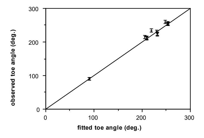
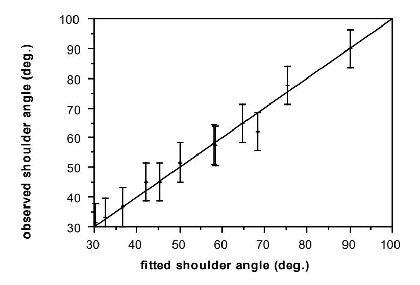
The fit of these equations to the observed data is shown graphically in Figures 3.13 and 3.14. Measurement error bars associated with a 95% confidence interval are also shown. The coefficient of determination (R2) for the data fit of each equation is given in Table 3.4.
| Angle | R2 | Degrees of Freedom |
|---|---|---|
| θS | 0.993 | 13 |
| θT | 0.990 | 13 |
3.4 VARIATION IN PARTICLE VELOCITY
3.4.1 Measurement Details
From the photographs taken of the charge fairly concentric streamlines were observed in the portion of the charge not in free flight, hereafter called the active part of the charge (see Figure 3.15). Measurements were made of the velocity of particles in each of these observed streamlines, whilst the position of each streamline was measured in terms of its radial displacement with respect to the centre of rotation of the mill.
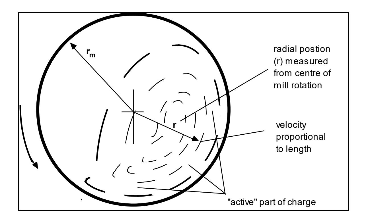
The measurements of the velocity of particles in the charge were normalized with respect to the mill shell speed. Similarly the radial positions of particles were normalized with respect to the mill radius. Pairs of data were therefore generated which comprised a normalized velocity (Vn) and an associated normalized radial position (Rn).
Hence $$ R_n = \frac{r}{r_m} $$
and $$ V_n = \frac{V_r}{V_m} $$
where
r = radial position
rm = mill radius at the mill shell liner wear face
Vr = tangential velocity at r
Vm = tangential velocity of the mill shell liner wear face.
Full details of these measurements are given in Appendix 2. These measurements were made directly off photographs of the charge using a steel rule. The precision of the technique was hence related to the resolution provided by the steel rule and the size of traces in the photograph. Using these criteria, the typical measurement error associated with the determination of the normalized velocity and position was estimated to be ±0.07 and ±0.01 (absolute) respectively.
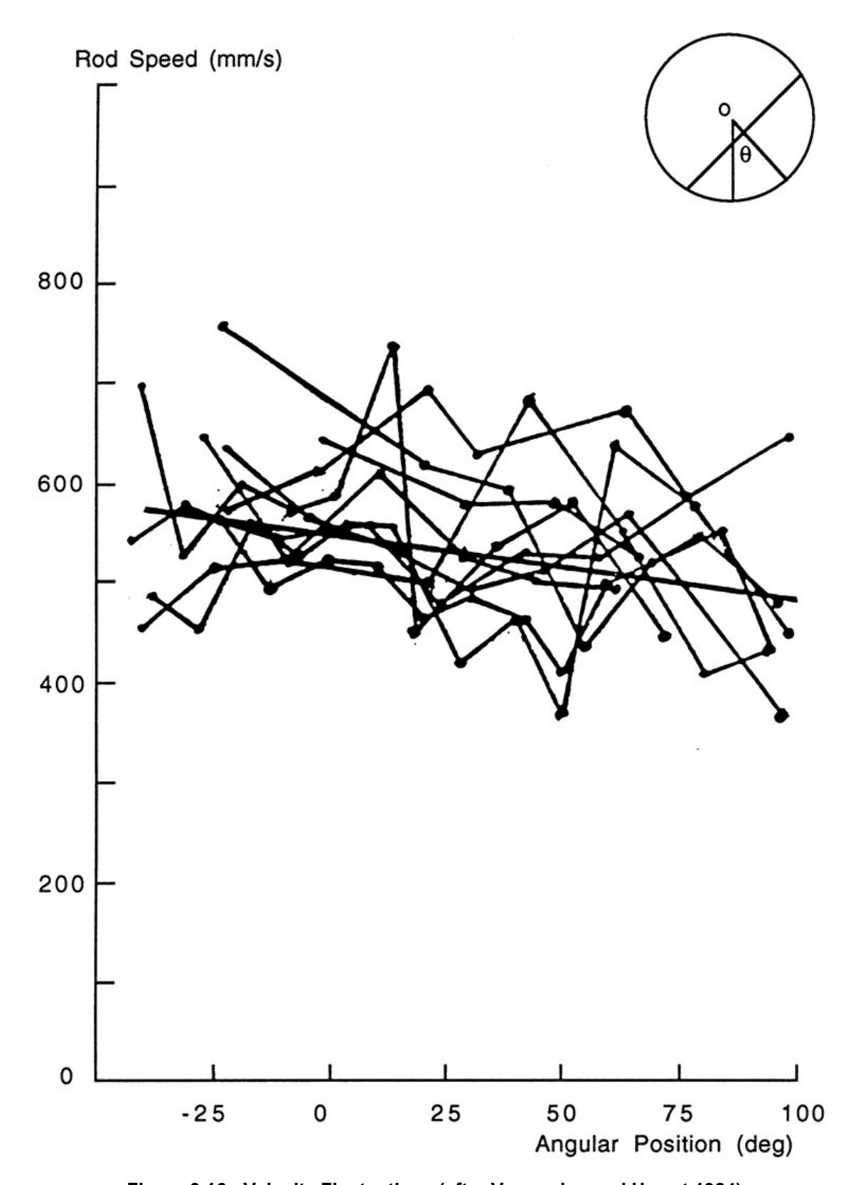
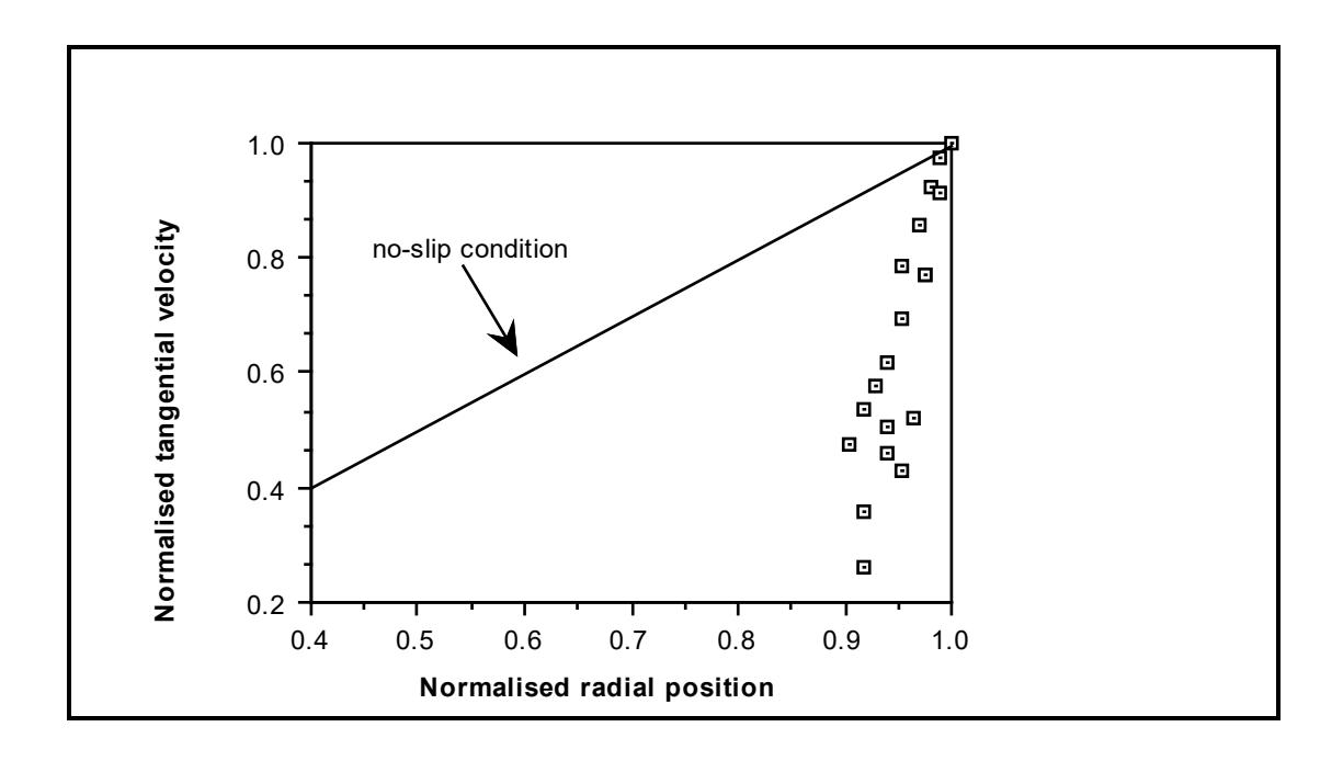
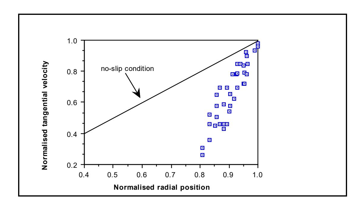
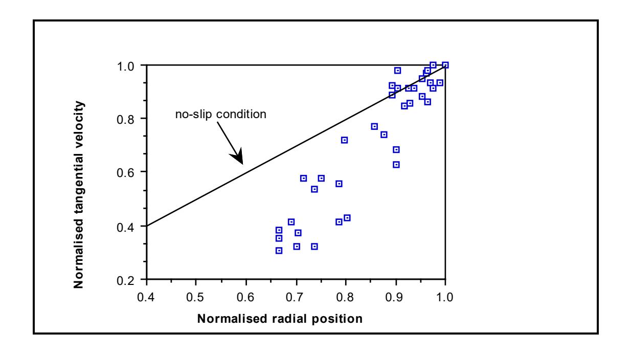
The data collected are plotted in Figures 3.17 - 3.19. It can be seen that despite some scatter an approximately linear relationship exist between Rn and Vn. The scatter is a result of the measurement technique employed and the likely variation in velocity along streamlines (Vermeulen and Howat, 1984). Vermeulen and Howat, although indicating that velocities along a streamline do vary, also showed that considerable velocity fluctuations at a given location occur (see Figure 3.16). From their data it would appear that fluctuations of local velocities are within the range of 15 - 20% of the mean value. With the techniques adopted in this work it was not possible nor desirable to track individual particles in a complete path around the mill to measure their velocities at each point. However, the objective of obtaining good estimates of the average velocity field was met and hence information on typical particle paths were deduced.
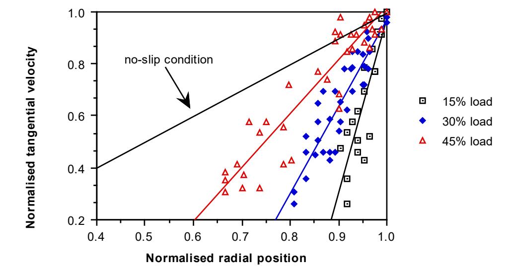
In order to compare the results obtained with different mill fillings Figure 3.20 shows the linear fits to the plots in Figures 3.17 - 3.19. It is apparent that an angular velocity gradient exists within the charge which is a function of mill filling. This is a direct result of slip occurring within the charge. As the friction force is proportional to the applied force acting in a direction normal to it, it is to be expected that the increased bed weights resulting from larger mill fillings will generate greater frictional forces within the charge. Less slip will therefore occur within the charge. Hence as the mill filling is increased the velocity gradient with respect to the mill radius will tend towards the no-slip condition.
3.4.2 Mathematical Description of the Velocity Profile
Linear regression analysis of the data from each mill filling resulted in equations 3.7 - 3.9 shown below. They provide a relationship between the mean tangential velocity along a streamline and the radial position of the streamline.
15% load:
$$ V_{n} = -5.7492 + 6.7194 R_{n} $$ (3.7)
30% load:
$$ R^2 = 0.821 $$ ; d.f. = 36
45% load:
R2 = 0.869; d.f. = 37 (3.9)
Equations 3.7 - 3.9 can be generalised in the form:
$$ V_n = (1 - A) + AR_n $$ (3.10)
where
A = a function of Jt.
Using the approximate relationship of A = Jt -1 produced the following equation:
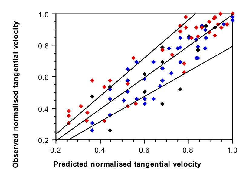
A plot using this equation to predict Vn is shown in Figure 3.21 together with the observed data. The velocity fluctuation limits as indicated by Vermeulen and Howat's work are also shown. It can be seen that the trends in the data are predicted very well. Scatter is apparent, however, but is of a similar magnitude to that seen in the graphs of Section 3.4.1.
3.5 CONCLUSIONS
Data were collected from a glass-ended laboratory mill using photographic techniques, which enabled the measurement of the variation in position of specific points in the charge as a result of changes in mill speed and mill filling. The same experiments yielded data on the change in angular velocity of particles, due to slip, which occurred within the charge itself. The change in velocity was seen to be a simple function of the mill filling. This is a natural consequence of the difference in the magnitude of the frictional forces which result from the different pressures that different loads impose.
Mathematically the variation in the toe and shoulder positions, as well as the velocity of particles within the charge, were adequately described using simple functions of the mill filling and mill speed. These equations are summarized as follows:
Toe Angle:
$$ \theta_{\rm T} $$ = 2.5307 (1.2796 - J t ) (1 - e -19.42 ( \( \phi_{\rm C} \) - \( \phi \) )) + \( \pi/2 \)
where
$$ \phi_{c} = \phi $$ ; \( \phi > 0.35 (3.364 - J_{t}) \)
$$ \phi_c $$ = 0.35 (3.364 - J t ) ; \( \phi \le 0.35 \) (3.364 - J t )
Shoulder Angle:
Normalized Tangential Velocity:
In the next chapter these equations will be used in a mathematical model of the theoretical power draw of cylindrical tumbling mills.
CHAPTER 4
MODELLING OF THE THEORETICAL POWER DRAW OF CYLINDRICAL TUMBLING MILLS
To provide a basis for a mathematical model of industrial grinding mills the simple case of a cylindrical tumbler is considered. Three different approaches are adopted to describe the theoretical power draw of such a vessel, based on the movement of the grinding media within it. A simplified charge shape is adopted for this purpose, whose position and velocity are described by the equations developed in Chapter 3.
4.1 INTRODUCTION
The power used to tumble a charge of rocks and/or balls in a rotating cylindrical vessel must be related to the motion and shape of the charge. A physical description of the charge shape and motion must firstly be made therefore. In the following sections a simplified charge shape is described which is subsequently used to develop theoretical equations which predict the power draw of tumbling mills.
These equations are devloped by considering three different approaches which describe the manner by which power is drawn by the mill viz.
- torque
- potential and kinetic energy balance
- friction force balance.
4.2 DESCRIPTION OF THE CHARGE SHAPE
To provide a description of the general shape of a mill charge which renders its mathematical treatment possible, yet at the same time reflects the essential shape which is observed in practice, the simplification shown in Figure 4.1 was assumed. From photographic evidence (see Figure 3.2) such a shape was considered more appropriate than the flat, inclined surface which has been the basis of most grinding mill power modelling over the last 30 years (Bond, 1961; Hogg and Fuerstenau, 1972; Harris and Arbiter, 1982; Austin, 1990).
The resistance that the mill motor feels to its rotation, and hence its power draw, is caused only by that part of the charge which exerts a force on the mill shell. The part of the charge which is in free flight, therefore, has no direct effect upon the mill. Similarly the material within the 'eye' of the charge, being effectively stationary and of relatively small mass, also has little effect on the mill power. Both these parts of the charge can therefore be ignored. Once this is done the remainder of the charge (the active charge) forms a crescent-like shape which is well approximated by Figure 4.1. In the following sections this charge shape is used to develop a simple model of the theoretical power draw of a cylindrical tumbling vessel.
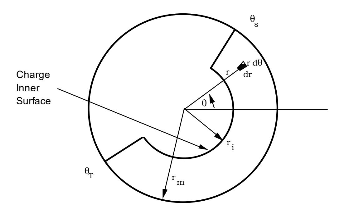
To describe the charge shape shown in Figure 4.1 the position of the shoulder, toe and charge inner surface must be known. The determination of these positions are described in the following sections.
4.2.1 Toe and Shoulder
The angular displacement of the shoulder and toe was described in Chapter 3 (equations 3.3 and 3.4). It is assumed that the boundary of the charge at the shoulder and toe is described by radial lines which start at the charge inner surface (see 4.2.2) and end at the mill shell.
4.2.2 Charge Inner Surface
The position of the charge inner surface is important in defining the limits of the charge. It can be represented by its radial distance from the axis of rotation (ri) (see Figure 4.1). If the location of the toe and shoulder are known, together with
the volume of the charge between these points, then \( r_i \) can be found from simple geometry:
$$ r_i = r_m \left( 1 - \frac{2\pi \beta J_t}{2\pi + \theta_S - \theta_T} \right)^{0.5} $$ (4.1)
where \( \beta \) is the fraction of the charge bounded by the toe, shoulder and charge inner surface, and the angles \( \theta_S \) and \( \theta_T \) are defined by equations 3.3 and 3.4.
As a first approximation \( \beta \) can be assumed to be equal to unity, in which case all the charge is considered to be contained between the toe, shoulder and the inner surface radius (Morrell, 1992). Some of the charge is in free-flight, however, and hence in reality \( \beta \) <1.
To estimate \( \beta \) it was assumed that it was related to the time taken for a particle to move between the toe and shoulder within the charge, and between the shoulder and toe in free flight. Hence:
where \( t_c \) = time taken to travel between the toe and shoulder within the active part of the charge
tf = time taken to travel between the shoulder and toe in freefall.
As there is an angular velocity gradient across the active part of the charge, \( \beta \) must be calculated using a mean value of the rotational rate ( Error! ) and mean radial position of the active charge ( Error! ). Hence the time taken to travel between the toe and shoulder within the active charge ( \( t_c \) ) is given by:
and the time taken to travel between the shoulder and toe in freefall \( (t_f) \) is given by:
As both Error!and Error!are themselves functions of \( r_i \) , this gives rise to a complex solution for equations 4.1 – 4.4. Error!and Error!can be approximated, however, by using the following relationships. These are based on the observed approximation that the rotational rate varies from \( N_m \) at the mill shell to zero at \( r_i \) . Error!is therefore approximately half of \( N_m \) and Error!is approximately half the sum of \( r_m \) and \( r_i \) :
$$ \overline{N} \approx \frac{N_{\rm m}}{2} $$ (4.5)
$$ \overline{r} $$ = \( \frac{r_{\rm m}}{2} \left[ 1 + \left( 1 - \frac{2\pi J_{\rm t}}{2\pi + \theta_{\rm S} - \theta_{\rm T}} \right)^{0.5} \right] \) (4.6)
By substituting equations 4.2 - 4.6 into equation 4.1, \( r_i \) can be estimated.
4.2.3 Velocity Profile
It was seen in Chapter 3 that there exists an angular velocity gradient within the charge which can be expressed as:
where
\( V_n \) = normalized tangential velocity
\( R_n \) = normalized radial position
A \( \approx J_t^{-1} \)
Equation 4.7 is needed to describe the change in velocity in the active charge between the inner surface radius (ri) and the mill shell radius(rm). As the mill filling increases the geometry of the active charge changes and the depth of the layer between \( r_i \) and \( r_m \) increases, giving rise to a higher charge pressure. This in turn causes higher frictional forces within the active charge, resulting in less slip and a change in the velocity gradient. This effect is reflected in equation 4.7 in the dependence of the parameter A on mill filling ( \( J_t \) ).
To relate the velocity gradient directly to the geometry of the active charge, rather than the mill filling, equation 4.7 was expressed in terms of the theoretical radius at which the velocity equals zero \( (r_0) \) . Subsequently \( r_0 \) was related to \( r_i \) and \( r_m \) . The advantage of this approach for modelling is that it ensures that the estimated velocity gradient is consistent with the estimated active charge geometry, both of which are dependent on the mill filling. This avoids the possibility of predicting negative velocities in the vicinity of \( r_i \) .
The approach taken is described in the following section.
Considering, firstly, the theoretical normalised radius at which the velocity equals zero ( \( R_0 \) ):
By setting the normalised tangential velocity to zero in equation 4.7, the parameter A can be expressed in terms of \( R_0 \) as follows:
Substituting for A in equation 4.7 gives:
Expressing equation 4.9 in terms of absolute values of velocity and radius gives:
Equation 4.10 can also be expressed in terms of the rotational rate, as the rotational rate \( (N_r) \) at radial position r is related to the tangential velocity \( (V_r) \) as follows:
Substituting equation 4.11 into equation 4.10 gives:
or
$$ N_{r} = \frac{N_{m}r_{m}(r - r_{o})}{r(r_{m} - r_{o})} $$ (4.12)
To incorporate the charge inner surface radius \( (r_i) \) in equation 4.12, \( r_i \) was related to \( r_o \) . The data shown in Table 4.1 were used for this purpose. The values for \( r_o \) were calculated using equation 4.7 for mill fillings of 0.15, 0.30 and 0.45, whilst mean values for \( r_i \) were measured from photographs of the charge in the laboratory glass mill.
| Fractional Mill Filling | r o | r i |
|---|---|---|
| (J t ) | (mm) | (mm) |
| 0.15 | 126.2 | 133.5 |
| 0.30 | 104.5 | 117.6 |
| 0.45 | 74.8 | 98.4 |
Using linear regression of a logarithmic transform of (1-Jt) and \( r_0/r_i \) the following relationship was developed:
$$ r_0 = (1 - J_t)^{0.4532} r_i $$ (4.13)
or
where
Table 4.2 shows how well equation 4.13 fits the data.
| Fractional Mill Filling | Fitted ro | Observed ro | |
|---|---|---|---|
| (Jt) | (mm) | (mm) | |
| 0.15 | 124 | 126.2 | |
| 0.30 | 100 | 104.5 | |
| 0.45 | 75 | 74.8 | |
Equation 4.12 thus becomes:
$$ N_{r} = \frac{N_{m} r_{m} (r - zr_{i})}{r (r_{m} - zr_{i})} $$ $$ (4.15) $$
4.3 THEORETICAL POWER DRAW EQUATIONS
Having defined the physical limits of the charge, equations were then developed which described the theoretical power draw associated with its observed motion. Three different methods for doing so were adopted. In each case it was assumed that once in free flight the energy of such particles was not recovered by the mill. This assumption is supported from photographic evidence over the normal operating range of industrial mills. It was found from these photographs (see examples in Figure 3.2 a-d) that at the point of impact at the toe, the particle trajectories were approximately radial and hence little tangential component was present. Only at very high speeds is this assumption less valid, as the extent to which energy recovery occurs increases as full centrifuging is approached. However, under conditions approaching centrifuging the energy of particles impacting at the toe was very small and hence the tangential component was likewise very small.
4.3.1 Torque Approach
In this approach the active charge within the mill is assumed to exert a torque acting against the rotation of the mill. The torque of each element of mass in the active charge is calculated and subsequently its associated power. The sum of all the powers associated with all elements of mass therefore gives the net power draw associated with the entire charge.
Consider an element of cross-sectional area dr rdθ and length L (see Figure 4.1). The mass of the element is given by:
where
$$ \rho_{c} $$ = charge density
and the torque exerted by the element is:
where
g = gravitational constant.
Power can be defined in terms of torque (τ) and rotation rate (N) as follows:
Power = $$ 2\pi N\tau $$
By integrating between the limits θS and θT and between ri and rm, the net power (Pnet) is given by
$$ P_{\text{net}} = 2\pi g L \rho_c \int_{r_i}^{r_m} \int_{\theta_T}^{\theta_S} N_r r^2 \cos\theta d\theta dr $$ (4.16)
where Pnet is the power delivered to the charge.
\( N_r \) is the rotational rate at radial position r. If the charge were locked and no slip occurred within it nor between it and the mill shell, \( N_r \) would remain fixed with respect to the radial position and would be equal to the rotational rate of the mill shell \( (N_m) \) . However, it was shown in Chapter 3 that slip occurs within the active charge giving rise to an angular velocity gradient across the charge.
From equation 4.15 this was represented as:
Substituting for \( N_r \) in equation 4.16 gives
The integral in equation 4.17 was evaluated by hand and checked using the mathematical package - 'Maple' (Char et al , 1991). The following expression was obtained.
$$ P_{\text{net}} = \frac{\pi g \, \text{L} \rho_{\text{c}} \, N_{\text{m}} \, r_{\text{m}}}{3 (r_{\text{m}} - z r_{\text{i}})} \left\{ 2 r_{\text{m}}^{3} - 3 z r_{\text{m}}^{2} r_{\text{i}} + r_{\text{i}}^{3} \left( 3 z - 2 \right) \right\} \left\{ \sin \theta_{\text{S}} - \sin \theta_{\text{T}} \right\} $$ (4.18)
4.3.2 Energy Balance Approach
In this approach the rate at which potential and kinetic energy is generated within the charge is considered. As power can be defined as energy per unit time, then the rate at which potential and kinetic energy is generated within the charge will provide an estimate of the mill power draw.
With reference to Figure 4.2, consider an element within the surface ABCD of length L and width dr. Its area is given by:
L dr
The tangential velocity of particles travelling through this surface is Vr and hence the volumetric flowrate through the surface is:
and the mass flow rate is:
The path of particles travelling through the element of surface is assumed to be as shown in Figure 4.2. Thus the rate at which potential energy is imparted to them is given by:
where the height difference (h) is given by:
The rate at which kinetic energy is imparted to the particles is given by:
Assuming that none of the energy of particles passing through surface ABCD is subsequently recovered by the mill, then the sum of the rate at which potential and kinetic energy is generated for all particles passing through surface ABCD (Pnet) is given by:
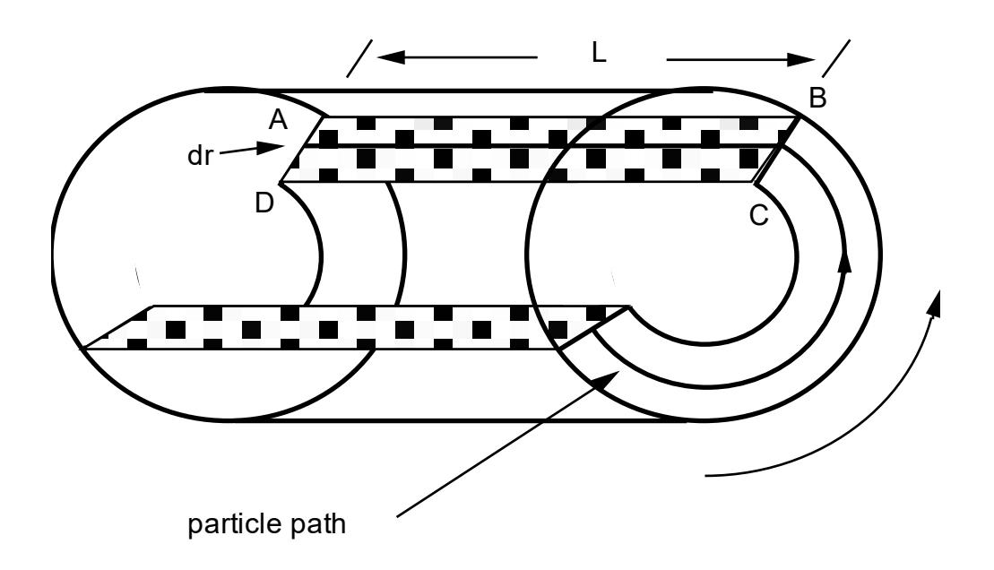
Expressing \( V_r \) in terms of \( N_r \) using equation 4.11 gives:
From equation 4.15, \( N_r \) can be expressed as:
Hence substituting for \( N_r \) in equation 4.20 gives:
$$ \frac{4\pi^3 \operatorname{L}\rho_{\rm c} \operatorname{N}_{\rm m}^3 \operatorname{r}_{\rm m}^3}{(\operatorname{r}_{\rm m} - z \operatorname{r}_{\rm i})^3} \int_{\operatorname{r}_{\rm i}}^{\operatorname{r}_{\rm m}} (\operatorname{r} - z \operatorname{r}_{\rm i})^3 d\operatorname{r} $$ (4.21)
+ $$ L\rho_c \left\{ \frac{N_m r_m \pi}{(r_m - z r_i)} \right\}^3 \left\{ (r_m - z r_i)^4 - r_i^4 (z - 1)^4 \right\} $$ (4.22)
It can be seen that the first term in equation 4.22 (the potential energy term) is identical to the power equation developed using the torque approach (equation 4.18). Equation 4.22, however, includes an additional term which describes the kinetic energy that requires to be supplied to the charge.
4.3.3 Friction Force Approach
The charge in a mill can only be moved by the transfer of energy from the rotating mill shell. As the only means of transferring that energy is via the friction forces acting between the mill and the charge, and within the charge itself, a friction force balance was considered.
It was assumed that along a streamline at radial distance r, the tangential velocity of a particle remained at a constant value \( (V_r) \) . Thus for the element shown in Figure 4.3, the component of its weight (W) acting tangentially must be balanced by a net frictional force (F) acting in the opposite direction. As power can be defined as the product of force and velocity, then the power required to move the element at velocity \( V_r \) , against the frictional force F, is given by:
\( V_r L\rho_c rg \cos\theta d\theta dr \)
By integrating between the limits θS and θT and between ri and rm, net power (Pnet), is given by:
$$ P_{\text{net}} = gL\rho_c \int_{r_i}^{r_m} \int_{\theta_T}^{\theta_S} V_r r \cos\theta \, d\theta \, dr $$ (4.23)
Expressing Vr in terms of Nr (equation 4.11) gives:
$$ P_{\text{net}} = 2\pi \, \text{gL} \, \rho_{\text{c}} \int_{r_{\text{i}}}^{r_{\text{m}}} \int_{\theta_{\text{T}}}^{\theta_{\text{S}}} N_{\text{r}} \, r^{2} \cos\theta \, d\theta \, dr $$ $$ (4.24) $$
It can be seen that this is the same expression for Pnet that was obtained using the torque approach (equation 4.16). Once again, as with the torque approach, the power required to provide kinetic energy is not included.
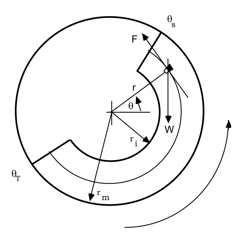
4.4 CONCLUSIONS
Based on the simplifying assumptions made about the shape of the charge in a cylindrical tumbling vessel and the velocity of particles within it, theoretical power draw equations were developed using 3 different approaches. The torque and friction force approaches provided identical results. Both these methods, however, over simplified the conditions prevailing in the mill and failed to account for the kinetic energy that the mill needs to provide the charge after it is brought to rest at the toe. It was found, therefore, that the torque and friction force equations were identical to the potential energy term only in the energy balance approach.
To provide a basis for the development of an industrial grinding mill power model it was decided to use the more comprehensive energy balance based equation. This is summarized as follows:
$$ \begin{array}{lll} \therefore & P_{net} & = & \frac{\pi g \; L \rho_c \; N_m r_m}{3 \; (r_m - z r_i)} \; \left\{ 2 r_m^3 - 3 z r_m^2 r_i + r_i^3 \; (3 z - 2) \right\} \; \left\{ \sin \theta_S - \sin \theta_T \right\} \; + \\ & + & L \rho_c \; \left\{ \frac{N_m r_m \pi}{(r_m - z r_i)} \right\}^3 \; \left\{ (r_m - z r_i)^4 - r_i^4 \; (z - 1)^4 \right\} \end{array} $$ where \( z = (1 - J_t)^{0.4532} \)
In all of the 3 approaches used, the power draw was related to the visible results of energy transfer from the mill shell to the charge ie. the motion and position of the charge. It was seen in Chapter 3 that an angular velocity gradient exists within the charge. This gradient is a result of slip between the particles of the charge. The relative motion of these particles will therefore give rise to the generation of heat due to friction and/or attrition and abrasion breakage of the rock charge. This 'invisible' energy, which can be regarded as internal losses, must be ultimately provided by the mill motor, but is not accounted for in any of the 3 approaches described in this Chapter, i.e. the energy dissipated as heat due to friction, breakage etc. in the process of raising the charge has not been considered. In addition, some rotational motion of the grinding media may occur. The energy to provide this motion has also not been incorporated in the equations. It is to be expected, therefore, that when applied to real milling systems these equations will underestimate the power drawn by the mill.
CHAPTER 5
A MODEL OF THE POWER DRAW OF CONTINUOUS INDUSTRIAL TUMBLING MILLS
In Chapter 5 the differences between an industrial grinding mill and a simple cylindrical tumbling vessel are described. These are principally the conical shaped ends of some mills and the discharge mechanism ie. overflow or grate. The equations for describing the power draw of the conical ends in a mill are shown to be extensions of those for the cylindrical section. To describe the power draw of overflow or grate discharge mills an additional term is required which describes the effect of a slurry pool (or absence of one) in the toe region. Finally, power losses due to bearing friction, motor and drive train inefficiencies are also described through an empirical relationship obtained from mills operated under no-load conditions (ie. empty).
5.1 INTRODUCTION
The equations developed in Chapter 4 related to a simple cylindrical tumbling vessel. Industrial mills are found to have a variety of shapes which, although they always include a cylindrical section, can have conical shaped ends whose associated power draw will be different to a simple cylinder. In addition the discharge mechanism is known to affect power draw (Bond, 1962; Morrell, 1992) and hence must have an effect on the charge which requires to be described by the model. Power must also be provided to overcome mechanical losses in the drive train, bearing friction losses and electrical inefficiences. A description of this power must also be incorporated within the model. In this chapter the incorporation of these factors in the basic power model is described.
5.2 MODEL STRUCTURE OVERVIEW
To put the ensuing sections of this chapter into context, a broad overview of the structure of the model is shown in Figure 5.1. The model consists of a number of levels. At the first level the gross power ie. the input power to the mill motor, is divided into that which overcomes mechanical and electrical inefficiencies from that supplied to the charge (net power). This is expressed as follows:
Gross Power = No-load Power + $$ (K \times Net Power) $$ (5.1)
where gross power = power input to the motor i.e. metered power
no-load power = power input to the motor when the mill is
net power = theoretical power transmitted to the charge to
K = calibration factor which accounts for heat
losses due to internal friction, energy
for attrition/abrasion breakage
and rotation of the grinding media.
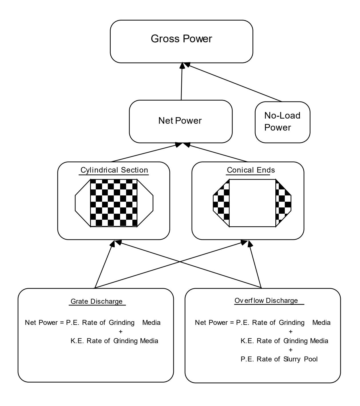
The net power in equation 5.1 is itself the sum of a number of separate terms, each of these terms describing a design characteristic of the mill. Thus depending on the design of the mill, the net power will be divided into the power contributed by the following:
- cylindrical section of the mill; grate discharge
- conical end section of the mill; grate discharge
- cylindrical section of the mill; overflow discharge
- conical end section of the mill; overflow discharge.
Despite the number of components to the model, it is true to say, however, that each term stems from a single, general equation for predicting the power draw in a simple cylindrical tumbling vessel.
5.3 INDUSTRIAL TUMBLING MILL DESIGN AND OPERATION
The most popular designs of industrial tumbling mills can be broadly classified according to the shape of their shell and the type of discharge mechanism that they use. Hence shell designs are either effectively cylindrical or incorporate conical ends (Figure 5.2), whilst discharge mechanisms are either overflow or have a grate arrangement (Figure 5.3).
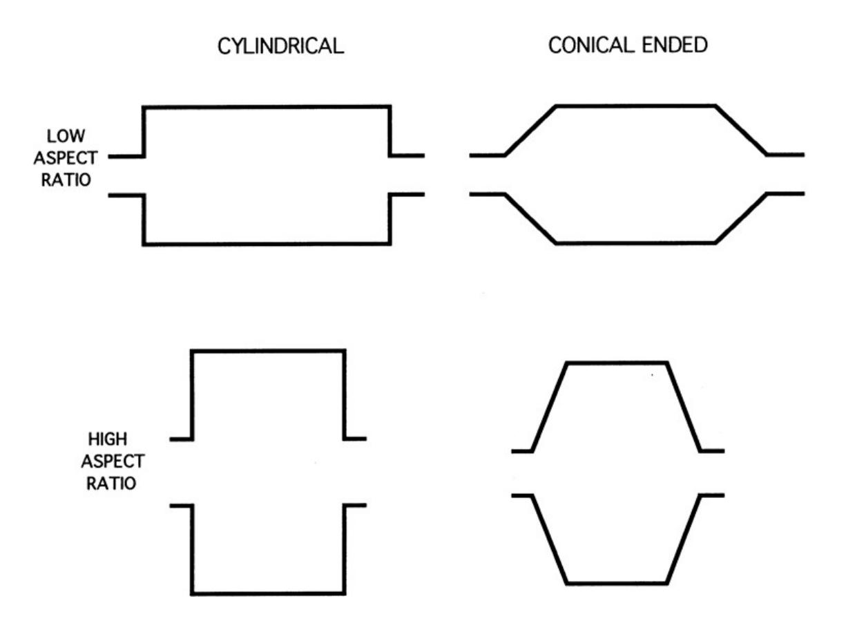
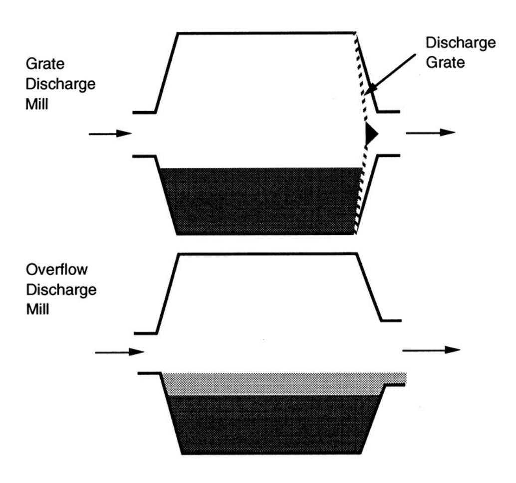
Operationally, tumbling mills typically fall into 4 classes viz:
- Autogenous
- Semi-autogenous
- Rod
- Ball.
Autogenous (AG) mills run with a rock and water charge only, and typically treat coarse feed such as that produced by a primary crusher or even uncrushed material directly from the pit. The discharge mechanism, is as far as the author is aware, exclusively of the grate type. Loads in the mill will vary depending on feedrate, ore hardness and feed size distribution.
Semi-autogenous (SAG) mills are variants of autogenous mills but are loaded with a ball charge typically in the range 0 - 12% (bulk volume). Charges of over 20% are sometimes used, however. The feed size range of SAG mills is greater than that of AG mills and may be fed secondary crusher product. Mill filling, as with autogenous mills, will vary depending on feed conditions.
Rod mills are used in a primary grinding role following secondary crushing. They have been largely replaced in Australia, however, by SAG and AG mills.
Ball mills are often found in secondary and tertiary grinding duties following a rod mill or AG/SAG mill. However, some are used in a primary duty following secondary or tertiary crushing. Ball mills are most often charged with balls to a filling level in the range 35 - 45%. Some primary mills, however, are run with lower charges down to the 20% level. The discharge mechanism is usually of the overflow type though some grate discharge designs are in operation.
The other main differences between mills are their speed of rotation and the shape, height and material of their lifters. Speeds can vary from as low as 65% of critical to 90% of critical. Lifters have a profusion of styles too numerous to mention. As a very general rule AG and SAG mills tend to be operated with higher profile lifters, whilst ball mills have lower profile lifters. It should be noted, however, that there are many exceptions to this rule.
It is the author's contention that the same model should be able to accurately predict the power draw of all the common industrial tumbling mill variants currently operated world wide. This assertion is based on the fact that in essence they are all approximately cylindrical in shape and, with the exception of rod mills, contain a collection of approximately spherical particles which are tumbled in the same predictable paths. If axial mixing effects are ignored then even rod mills should have a similar charge pattern to that of ball and AG/SAG mills, as the two-dimensional cross sections are the same.
In summary, the effects of mill design and operation with respect to power can be reduced to consideration of the following:
- Mill speed this will affect the rate at which energy is imparted to the charge as well as the position of the toe and shoulder.
- Mill filling changes in filling will change the mass of charge which has to be moved by the mill. The position of the toe and shoulder will also vary.
- Charge density due to differences in density of different ores and the much higher density of steel balls/rods, AG, SAG, rod and ball mills will have different charge densities.
- Grate and overflow discharge overflow mills will contain a slurry pool which an efficient grate discharge mill will not. Charge shapes in the toe region will therefore be different in each case.
- Cylindrical or conical end sections a mill with conical ends will hold additional media and slurry, which in turn will result in a higher power draw than a cylindrical mill with the same dimensions as the cylindrical section of the conical-ended unit.
- Lifter type different lifter profiles/heights will change the amount of lift given to the charge in contact with the lifters.
Using the energy balance approach described by equation 4.22 (see Section 4.3.2) as its basis, the remainder of this chapter is devoted to developing equations to describe the above 6 factors. Rod mills will not be considered in this analysis due to their increasingly rare occurrence in the Australian minerals processing industry, and consequent lack of substantial data on their operation. It is expected, however, that the only change necessary to the equations describing AG/SAG and ball mills will be in the charge density, which will be higher in rod mills (Rowland, 1972).
5.4 MILL SPEED
Mill speed is either quoted in terms of rpm or, more commonly, % of critical speed. Critical speed is the theoretical rate of rotation of a mill at which centrifuging of the charge will commence. At this point centrifugal forces balance gravitational forces and hence:
$$ \frac{v_c^2}{r} $$ = g
where
vc = critical tangential velocity
r = radius
g = gravitational constant.
therefore
The % of critical speed is a useful term for comparing speeds of different mills as it is independent of radius. A natural consequence of mills running at the same % of critical speed is that for the same mill filling the relative time spent by particles in the active charge and in free-flight remains the same regardless of mill diameter. This can be shown from the following analysis:
For a given % of critical speed the tangential velocity (v) at diameter, D, is given by:
The time taken to travel in the active charge between a given toe and shoulder position (tc) is therefore given by:
Therefore:
For a given particle in free flight undergoing constant acceleration, the time taken to travel between the shoulder and toe (tf) is given by:
The ratio of tc/tf is therefore independent of diameter.
As the amount of material in the active charge and in free-flight is proportional to the time spent in each (section 4.2.2), then the relative amount of material in each region will also be independent of mill diameter. Thus the pattern of the mill charge revolving inside the mill should be the same in mills running at the same % of critical speed regardless of their diameter. It was seen in Chapter 3 that the toe and shoulder angles vary as mill speed varies and that the relationship between speed and these angles is also a function of the mill filling. As the toe and shoulder angles vary, so will the power draw, due to changes in the potential energy between both positions. In addition, the speed has a direct effect on power due to its influence on the rate at which potential energy is imparted to the charge ie. the frequency with which the charge is turned over inside the mill. The effect is best illustrated using the torque-based definition of power:
Power = 2π Nτ
where
τ = torque
N = mill speed (rpm).
The power model thus takes account of speed effects through the empirical relationships developed between the fraction of critical speed and the toe and shoulder angles, plus the direct effect caused by changes to the rate of rotation of the charge.
5.5 MILL FILLING
Mill filling is the fraction of the total mill volume that is occupied by the charge. In Chapter 3 the toe and shoulder position were found to vary as the mill filling was varied. This response was found to be speed dependent such that centrifuging commenced at lower speeds as the mill filling was increased. In addition to the toe and shoulder position changing, the charge inner surface radius also changed. This is a natural consequence of the change in charge volume as the mill filling is changed.
The other influence of mill filling was found to be on the angular velocity gradient. Higher mill fillings result in higher charge pressures with resultant higher frictional forces. These higher frictional forces discourage slip within the charge and give rise to the observed trend that as the mill filling increases the angular velocity gradient within the charge tends to the no-slip condition.
All of the above effects are explicitly incorporated in the model via equations relating the toe and shoulder angles, the angular velocity gradient, and the charge inner surface radius to the mill filling.
5.6 CHARGE DENSITY
As the ore s.g. (ρo), ball s.g. (ρB), and the relative amounts of steel balls, ore and water vary, so will the charge density (ρc). The following assumptions were made concerning these factors:
- In AG, SAG mills and primary ball mills the ore charge comprises two components - a coarse fraction and a slurry which can fit within the interstices of the coarse fraction (and ball charge where it exists).
- The coarse ore fraction has a bed porosity (E) similar to that of a charge of steel balls.
- The slurry fraction has a fractional solids content by volume (S) equal to the mill discharge slurry.
- In secondary and tertiary ball mills only the ball bed and slurry fraction are assumed to exist.
- The voidage in the coarse ore/ball bed is occupied by slurry; the fraction of the voidage occupied by slurry is denoted by U.
On the basis of these assumptions the following equations were developed.
The mass of coarse ore is:
$$ \pi r_{\rm m}^2 \ L(J_{\rm t} - J_{\rm B}) \ (1 - E)\rho_{\rm o} $$ (5.2)
where
Jt = fraction of the mill volume occupied by the entire charge (including voids)
JB = fraction of the mill volume occupied by balls (including voids)
rm = mill radius inside the liners
L = mill length inside liners.
The mass of the slurry fraction is:
$$ \pi r_{\rm m}^2 \, LJ_{\rm t} \, EUS\rho_{\rm o} $$ (5.3)
The mass of water is:
$$ \pi r_{\rm m}^2 \ LJ_{\rm t} \, EU(1-S) $$ (5.4)
and the mass of the balls is:
$$ \pi r_{\rm m}^2 \ LJ_{\rm B} (1 - E) \rho_{\rm B} $$ (5.5)
Therefore, the total charge mass is:
$$ \pi r_{\rm m}^2 \ L \left[ J_{\rm t} \rho_{\rm o} \left( 1 - E + EUS \right) + J_{\rm B} \left( \rho_{\rm B} - \rho_{\rm o} \right) (1 - E) + J_{\rm t} EU (1 - S) \right] $$ (5.6)
The charge density (ρc) is thus given by:
and
The fraction of the mill occupied by the entire charge of balls and coarse ore, (Jt), and the fraction of the mill occupied by balls (JB), must be known, together with the fraction of the charge voidage occupied by slurry (U), voidage (E) and the discharge slurry fractional solids content (S).
In the absence of data for E, U and S values of 0.4, 1 and 0.5 respectively, can be assumed. In this case equations 5.7a and 5.7b simplify to:
$$ \rho_{c} = 0.8\rho_{o} + \frac{0.6 J_{B}(\rho_{B} - \rho_{o})}{J_{t}} + 0.2 $$ (5.8)
5.7 OVERFLOW AND GRATE DISCHARGE MECHANISMS
5.7.1 General Shape of the Charge
In a grate discharge mill the charge typically runs with the interstices in the grinding media (coarse) fraction rarely filled much beyond the point where all the voidage is occupied with slurry. The charge in such mills can be approximated as shown in Figure 5.4a. In the case of an overflow discharge mill slurry can only discharge once it overflows the discharge trunnion. Excess slurry is therefore present and gives rise to the second charge shape shown in Figure 5.4b. In this case a slurry pool exists in addition to the grinding media. The slurry pool is assumed to comprise a mixture of ore and water of the same density as the discharge slurry. The remainder of the charge is assumed to comprise the media whose interstices are fully occupied by slurry at the same density as the discharge slurry.
The presence of the slurry pool in the overflow mill results in a reduction of the power draw of the mill when compared to a grate discharge unit of the same size. In an empirical manner such differences in power draw have been incorporated in some mill power equations (Bond, 1962; Morrell, 1992). Mechanistically this effect can be considered to be caused by the assistance to rotation that the slurry in the toe region provides. Only the toe region needs to be considered as far as the power draw is concerned. The symmetrical portion of the slurry pool lying vertically beneath the centre of rotation of the mill can be assumed not to exert a torque and hence does not contribute to the net power draw of the mill. However, it will provide an additional mass which, through increased frictional forces at the mill bearings, will cause an increase in mechanical losses. The magnitude of this effect, however, is considered to be small.
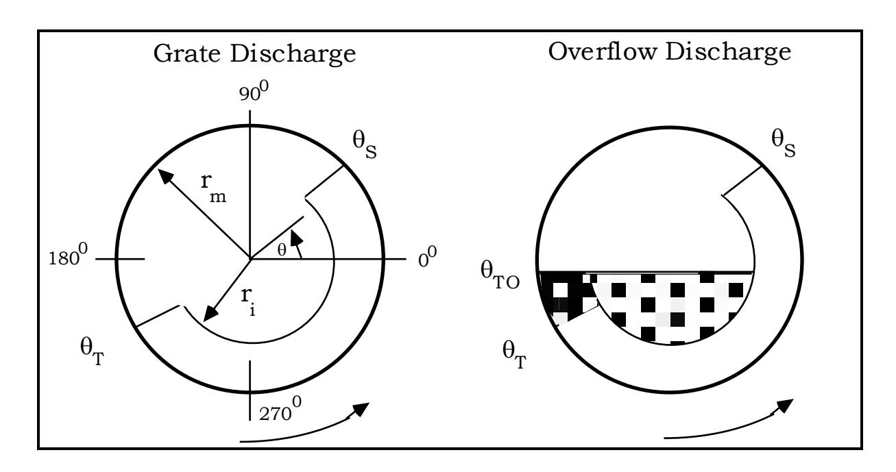
Figure 5.4b: Simplified Charge Shape for Overflow Mills
5.7.2 Power Draw Equations
Equation 4.22 was derived assuming the charge shape shown in Figure 5.4a and is hence applicable to grate discharge mills. For overflow discharge mills, the effect of the slurry pool must be incorporated by an additional term which describes the rate at which it provides potential energy to the mill. The form of this equation is the same as the potential energy part of that for the grinding media charge (equation 4.19). The charge density, however, is assumed to be that of the discharge slurry, and the toe limits are between \( \theta_T \) and \( \theta_{TO} \) (see Figure 5.4b). Hence the power associated with the toe ( \( P_{\text{net-toe}} \) ) is given by:
$$ P_{\text{net-toe}} = \int_{r_i}^{r_m} V_r L\rho_p \, rg \, (\sin\theta_T - \sin\theta_{TO}) \, dr $$ $$ r_i $$ (5.9)
On evaluating the integral in equation 5.9 it reduces to the following:
$$ P_{\text{net-toe}} = \frac{\pi g L \rho_p N_m r_m}{3 (r_m - z r_i)} (2 r_m^3 - 3 z r_m^2 r_i + r_i^3 (3 z - 2)) (\sin \theta_T - \sin \theta_{TO}) $$ (5.10)
Equations 5.10 and 4.22 can now be expressed in the following single equation which describes both grate and overflow mills:
where
\( \rho_p \) = discharge slurry density
\( \rho_c \) = grinding charge density
\( \theta_{TO} \) = slurry toe angle for overflow discharge mills and
\( \theta_{TO} = \theta_T \) for grate discharge mills
5.7.3 Determination of the Position of the Slurry Toe ( \( \theta_{TO} \) )
The position of the slurry pool, as measured by the angle \( \theta_{TO} \) , can be calculated theoretically from a knowledge of the trunnion diameter, mill diameter and slurry level within the mill.
The slurry level will vary with throughput, a higher level resulting from a higher throughput. The slurry level can be estimated by making the simplifying assumption that the discharge trunnion behaves like a rectangular section, broad crested weir (Figure 5.5).
By applying the Benoulli equation to such a weir of width b, then the velocity (u) at the end of the weir can be obtained by solving (Kay and Nedermann, 1974):
The volumetric discharge rate (Q) is therefore given by:
$$ Q = b\lambda(2g)^{0.5} (h-\lambda)^{0.5} $$ (5.12)
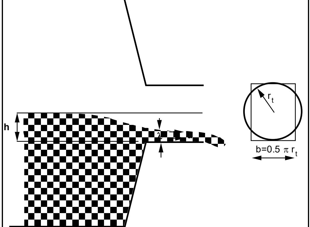
For maximum discharge
$$ \frac{dQ}{d\lambda} $$ = 0 at constant h
By differentiating equation 5.12 and setting dQ/dλ to zero gives:
By substituting for \( \lambda \) in equation 5.12 therefore gives:
$$ Q_{\text{max}} = bg^{0.5} (0.67h)^{1.5} $$ (5.13)
To maintain the same cross-sectional area and maximum vertical height as the mill discharge trunnion, b must be set to \( \pi r_t/2 \)
Hence $$ Q_{\text{max}} = 0.5 \, \pi r_t \, g^{0.5} \, (0.67h)^{1.5} $$ (5.14)
or h = $$ 0.67 \left( \frac{2Q}{\pi r_t g^{0.5}} \right)^{2/3} $$ (5.15)
With reference to Figure 5.6, \( \theta_{TO} \) can be calculated as follows:
$$ \theta_{\text{TO}} = \arcsin\left(\frac{r_{\text{t}} - h}{r_{\text{m}}}\right) + \pi $$ (5.16)
By substituting equation 5.15 into equation 5.16, \( \theta_{TO} \) can be found.
As a rule of thumb (Hadaway, 1992) the trunion diameter is approximately 0.25D. Hence from equation 5.16:
$$ \theta_{TO} $$ < arc sin (0.25) + \( \pi \) or \( \theta_{TO} \) < 3.395
In the absence of data on Q (and hence h) therefore, a value of 3.395 for \( \theta_{TO} \) can be used.
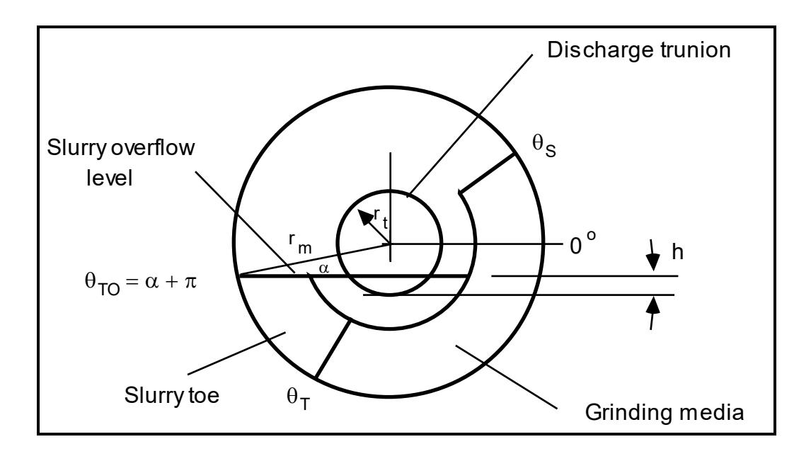
5.8 CONICAL END SECTIONS
Some mills, particularly those with large diameter to length ratios, are not completely cylindrical, but have conical shaped ends (Figure 5.2). The charge shape in such mills is assumed to be as shown in Figure 5.7. For simplicity only the grate discharge mill shape is shown.
It is assumed that the position of the toe and shoulder is the same in the cone ends as in the cylindrical section. As the amount of charge in the cone-ends is typically quite small, it is assumed that the keying effect of the end lifters will limit slip within the cone-end charge. For this reason it is assumed that there will be no angular velocity gradient within this part of the charge.
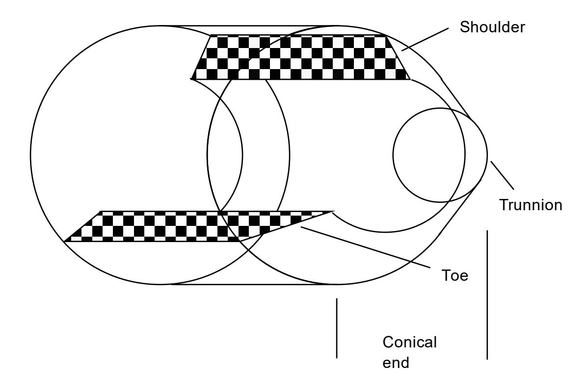
With reference to Figure 5.8, for an element of length \( dL_c \) within the cone section, the power draw equation will have the same form as for a cylindrical vessel (equation 4.19). Hence for the element of length \( dL_c \) at a cone radius of \( r_c \) , the power draw ( \( P_{dLc} \) ) for a grate discharge mill will be given by:
$$ P_{dLc} = dL_c \int_{r_i}^{r_c} \left\{ V_r \rho_c rg \left( sin\theta_S - sin\theta_T \right) + \frac{V_r^3 \rho_c}{2} \right\} dr $$ (5.17)
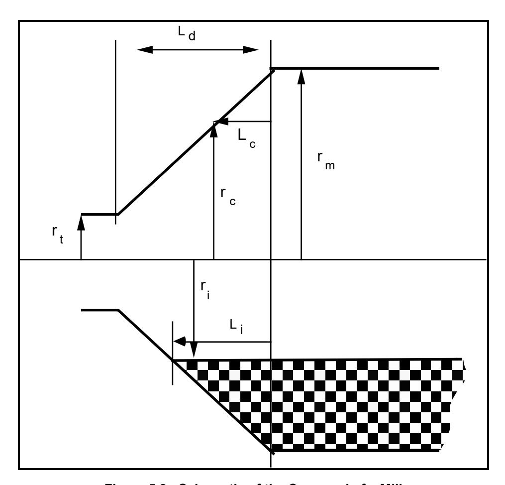
Expressing \( V_r \) in terms of \( N_m \) gives
Substituting for \( V_r \) in equation 5.17 gives:
As the radius of the cone varies with respect to its length, then for the entire cone equation 5.18 must be integrated with respect to the cone length \( L_c \) . Hence the total power associated with both cone ends ( \( P_c \) ) is given by:
From geometry
$$ L_{c} = \frac{(r_{m} - r_{c})}{(r_{m} - r_{t})} L_{d} $$ (5.20)
$$ \therefore dL_c = \frac{-L_d dr_c}{(r_m - r_t)} $$ (5.21)
By substituting equation 5.21 into equation 5.19 gives:
$$ 4\pi^{3} N_{m}^{3} \rho_{c} \int_{r_{i}}^{r_{m}} \frac{1}{4} (r_{c}^{4} - r_{i}^{4}) dr_{c} \} $$ $$ = \frac{2L_{d}}{(r_{m} - r_{t})} \left\{ \frac{1}{6}\pi N_{m} \rho_{c} g(\sin\theta_{S} - \sin\theta_{T}) (r_{m}^{4} - 4r_{m} r_{i}^{3} + 3r_{i}^{4}) + \frac{1}{5} \pi^{3} N_{m}^{3} \rho_{c} (r_{m}^{5} - 5r_{m} r_{i}^{4} + 4r_{i}^{5})) \right\} $$ (5.22)
Using the same approach as adopted for the cylindrical section, equation 5.22 can be extended to encompass overflow mills as follows:
5.9 NO-LOAD POWER
To be practically useful a power model needs to predict accurately the gross (ie. metered) power. The difference between gross and net power draw in a mill is due to losses associated with various electrical and mechanical components. The main losses occur in the motor, gearing and bearings. None of these remains constant over the mill's full operating range. Some, however, may have a fixed component - for example, losses in the bearings due to friction will be dictated by the weight of the mill when empty (a fixed component, though even this will vary as liners and lifters wear) and the weight of the mill charge (a variable component).
In most, if not all, full-scale operating plants the only data that will be measured is gross power and/or current. In rare cases no-load power (the gross power drawn by the mill when running empty) will be known from commissioning records. Alternatively, if the mill has been emptied for relining, the no-load power is sometimes recorded at start-up. Such data indicate the magnitude of some of the power-loss components which are typically close to a constant value.
To determine the relationship between no-load power and mill design parameters, 14 data sets were analysed from 12 mills with diameters ranging from 1.8 to 9.75m. It was assumed that the no-load power was drawn principally to overcome bearing friction, which, in turn, was assumed to be proportional to the mill's weight when empty. The frictional force at the bearing acts at a distance equal to half the diameter of the trunnion. Therefore, on the basis that the weight of the empty mill is proportional to its volume and the diameter of the trunnion is proportional to that of the mill, it would be expected that the parameter D3 LNm is related to the no-load power. This parameter was therefore regressed against no-load power and found to provide a reasonable fit. Expressing mill speed in terms of the fraction of critical speed (ø), the relationship that was developed was:
No-load Power (kW) = $$ 2.62 (D^{2.5}L\emptyset)^{0.804} $$ (5.24)
The associated R2 value and degrees of freedom were 0.79 and 13 respectively.
It was apparent from data collected from 2 different pilot mills of very similar dimensions, that a fair degree of scatter existed in the no-load readings from each, with readings varying in the range 2.73 - 5.1kW. This was attributed to the differences in the condition of the bearings and mechanical drive train, plus the inaccuracies in measurements of the power draw. Using the scatter in these data as being indicative of the range of readings which might be expected in full scale plant, the standard deviation of observed measurements was estimated to be 26.7% of the mean value. At first sight this appears to be an unrealistically high error. However no-load measurements were obtained during commissioning of 2 identical new mills which gave readings of 507kW for one of the mills and 594kW for the other. Under such circumstances where the mills are new, differences between no-load readings should be at their absolute minimum. In this case the higher reading was 20% higher than the lower reading, which is of the same order of magnitude as the estimated standard deviation of readings obtained from the pilot mill. A plot of observed vs predicted no-load powers together with 95% confidence error bars is shown in Figure 5.9.
A further point should be mentioned concerning the conditions under which noload measurements are usually made. To prevent flywheeling and damage to the ring gear, mills are rarely run without at least some water in the mill. Some of the data which were recently collected by the author were from mills where water was known to have been added. Other data are historic and it is not known what the conditions were under which they were collected. Some of the so-called no-load power data presented in this section are therefore not truly the power drawn by the mill when running completely empty. It is the purpose of this work, however, to provide a useful mill model which can be calibrated using data which can be collected from operational mines. The data are the best available and although somewhat scattered, are considered adequate for the current study.
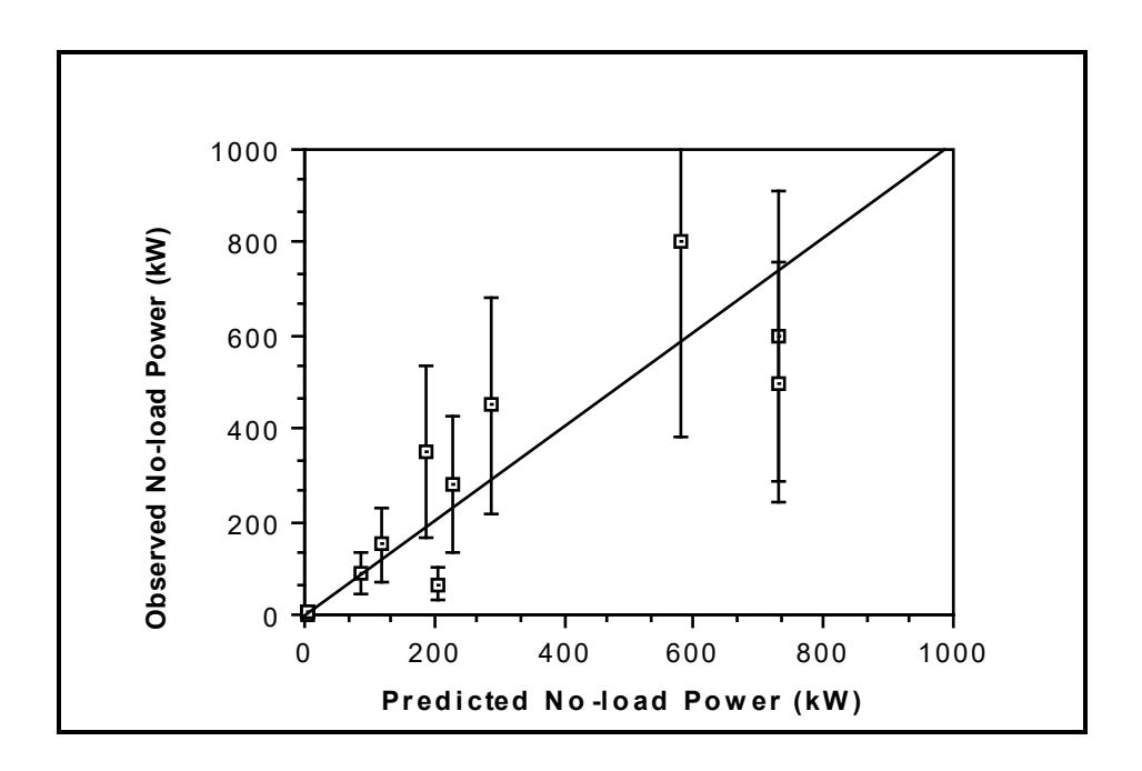
5.10 CONCLUSIONS
The general equation for the theoretical power draw of simple cylindrical tumbling vessels which was developed in Chapter 4, was extended to account for the machine design related effects of grate discharge mechanism and conical endshell sections. Operational differences such as are embodied in AG, SAG and ball mill variants were also described via equations describing the charge density. The effect of electrical and mechanical power losses was accounted for by an additional term which was determined from no-load power readings from a number of different mills.
The equations for predicting ball, SAG/AG mill power are summarized as follows:
Net Power of Cylindrical Section:
Net Power of Cone Ends:
No-Load Power:
No-load Power = \( 2.62 (D^{2.5}L\phi)^{0.804} \)
CHAPTER 6
INDUSTRIAL MILL DATA
To provide industrial data with which to validate a power model, a data collection exercise was mounted. This yielded a total of 76 data sets covering ball, SAG and AG mills in the power draw range 6.8 - 7900kW. Considerable efforts were made to ensure that the data were of good quality. Such efforts included direct measurement of charge levels, internal dimensions and verification of power draw readings. In the latter case this took the form of check calibrations by plant electrical staff and/or cross-checking with different instrument sources on the plant. In some instances inconsistencies were apparent which could not be resolved. In these cases such data were excluded from the data base.
6.1 INTRODUCTION
Although small laboratory mills provide an excellent test bed to determine the functional relationships between operating conditions and power draw, good quality full scale plant data are required to determine whether such relationships hold at the industrial level.
Some industrial mill data can be found in the literature. However these are isolated cases and often lack sufficient detail to be useful for research purposes. The problem is compounded by the inherent difficulties in obtaining accurate data (Harris et al, 1985). In 1988, therefore, the author began to assemble a grinding mill data base which could be confidently used to develop and validate mill power models. The following chapter provides details of the data base and describes the methodology of its construction.
6.2 DATA BASE STRUCTURE
The minimum detail required from a grinding mill to be able to predict its power draw is listed as follows:
- diameter (inside liners)
- length (inside liners)
- speed
- ball filling
- total filling (balls plus rock)
- discharge mechanism (grate or overflow)
- ore specific gravity.
These details, together with the true power draw, were therefore sought for a wide a range as possible of mill dimensions, ore types and operating conditions. Five sources for these data were used:
• field studies of industrial mills by the author
- field studies of industrial mills by students/staff under the author's direction
- archives at the JKMRC relating to field studies of past staff/students
- data provided by companies sponsoring JKMRC research programmes
- studies conducted by the JKMRC's commercial arm JKTech.
6.3 DATA ACCURACY
During the course of collecting power draw and associated data a variety of potential sources of error were encounted.
These included the following:
• Mill Diameter - it is a fairly common misconception amongst plant personnel that the dimensions quoted in manufacturers manuals are inside liners. In fact the dimension usually quoted by the manufacturers are inside shell. As a result many plant personnel when requested to provide inside liner details will provide those for the inside shell. Inside liner diameters can only be reliably obtained by direct measurement from inside the mill. In a number of cases the author was able to do this. However in some instances inside shell diameters only were available. In such cases two nominal half-worn liner thicknesses were subtracted from the inside shell dimensions.
The thickness of new liners varies with mill diameter, with small diameter mills having thinner sections. In addition, different mill suppliers and liner manufacturers will specify slightly different liner thicknesses. As a general rule, however (Hadaway, 1992), the following relationship can be used:
Mill Diameter Liner Thickness
2 - 4m 50 - 75mm
4 - 10m 75 - 125mm
A mathematical relation consistent with the above was used as follows:
Liner thickness (mm) = $$ 0.04 \times D^{0.5} $$ (6.1)
where D = mill diameter inside shell in metres
Where the actual mill diameter inside the liners was unable to be measured, the assumption of a half worn liner thickness could give rise to a maximum error on the true diameter measurement of 0.04 x D0.5 metres ie. the equivalent of a new liner thickness.
- Mill Length manufacturers will often quote an 'effective grinding length' (egl) for a mill. It is apparent that manufacturers differ in their definitions of what this is. In some cases it appears to be the length of the mill at the belly (ie. the cylindrical section), inside the shell. In conical ended mills this is misleading as it effectively ignores the mill volume within the conical ends. Some manufacturers take account of this by specifying an egl which is in between the belly length and the centre-line lengths. In such cases it has not been established how this length is determined. Wherever possible engineering drawings were sought and both belly and centre-line lengths determined. In some cases direct measurement was possible. Failing either of these, the manufacturers egl was used. As with the mill diameter, where actual measurements were not possible a nominal half worn liner thickness was assumed. The liner thickness was calculated using equation 6.1. The maximum error on the mill length associated with the assumption of half worn liners will also be equal to 0.04 x D0.5 metres.
- Mill Speed the most common method for reporting mill speed is the % of critical speed. This figure is often based on the rpm of the mill and a nominal inside liner dimension. As the % of critical speed is proportional to D0.5, the value calculated for the true inside liner dimension will therefore differ from this value. Wherever possible rpm data have been recorded and the % of critical speed at the inside of the liners then calculated.
Once again the maximum error on the critical speed calculation will be related to the error on the diameter measurement. As the critical speed is related to D0.5 the maximum error on the critical speed calculation will be:
max error =
$$ (D + 0.04D^{0.5})^{0.5} - D^{0.5} $$
=
\( D^{0.5} \{ (1 + 0.04D^{-0.5})^{0.5} - 1 \} \)
- Ball Specific Gravity different grades of steel and different ball manufacturing techniques result in varying ball specific gravities. No information was sought on ball sg during the course of this research and hence a mean sg of 7.8 has been used. In the literature ball sgs of up to 8.0 have been used (Austin, 1990). The use of 7.8 therefore may give rise to a maximum error of 0.2 sg units.
- Ore Specific Gravity in SAG and AG mills in particular, the ore sg has a significant effect on charge density and hence power draw. In all the data sets in the author's data base the mean feed ore sg has been used. It is possible, however, that where blends of ore are being treated a harder constituent may be present of different sg to the remaining ore. In which case the sg of the ore in the mill will be different to that of the feed ore.
- Mill Filling the mill filling is the volume of charge in the mill and hence has a significant effect on the power draw. In the case of ball mills the filling remains fairly steady over time, as it comprises mostly steel balls. It is common practice for operators to charge ball mills with steel balls according to a power set point. Due to the very stable power draws that are usually seen with ball mills, this procedure ensures that the mill is always charged to approximately the same level. In cases where direct measurements of the ball filling were not possible at the time when power readings were taken, plant historic records were used as a source for ball filling data. In AG/SAG mills, however, the feed ore contributes significant quantities of rock to the grinding media. As a result, changes in feed ore size distribution and hardness will affect the quantity of ore within the mill and hence the power draw. In all cases direct measurements of the loads were taken. In the case of AG/SAG mills this
entailed running the mills under steady state then crash-stopping them under load. Access to the mill was then gained through the feed trunnion after drawing back the feed chute. Due to production constraints, in some instances the author had to gain access down the feed chute whilst the feed chute was still in place. This latter procedure was found necessary to ensure direct measurements of the charge could be made. However, it is not to be generally recommended for reasons of safety. Once inside the mill, measurements of the width of the charge in 3 places were taken together with inside-liner dimensions. From these measurements the load volume was calculated using simple geometry (Appendix 3). In a number of cases access to the mill interior was denied. In such cases either photographs of the charge against the grate were taken and the charge level determined using engineering drawings of the grate and simple geometry. Alternatively a rod was inserted into the mill to measure the charge level below the feed trunnion.
SAG mill operations presented additional difficulties due to the ball filling which, being mixed with the ore charge, was difficult to estimate. In most cases mills were allowed to grind-out and the ball filling then measured. Due to the damage that this procedure can cause to the liners/lifters, however, this was not always possible. In such cases operator's estimates had to be used.
Typically plant operational staff have been found to favour the technique of measuring either the distance between the feed trunnion and the charge surface or the mill roof and charge surface. Using this measurement and simple geometry the mill filling can be calculated. Where data were donated by mining companies it was subsequently discovered that in some cases mill filling calculations had been made using the Allis Chalmer approximation rather than geometry. This approximation is as follows:
where
h = vertical distance between the charge surface and the mill roof, inside the liners.
D = mill diameter, inside the liners.
Although useful for relatively high mill fillings, this equation gives very large errors for smaller mill fillings. Figure 6.1 illustrates this in a plot of equation 6.1 against the true mill filling. In cases where this equation was used the values were corrected.
It is difficult to assess what were the measurement errors associated with the determination of mill filling. They will be related, however, to the accuracy in measuring either the charge width or height between the charge and mill roof. It is believed that these measurements should be capable of being made to within 50mm. On this basis, for a nominal mill filling of 30%, the maximum error using the technique shown in Appendix 3 will be related to the mill diameter as follows:
| Diameter | Error in Mill Filling | ||
|---|---|---|---|
| (m) | Estimate (%) | ||
| 2 | 9.62 | ||
| 6 | 3.43 | ||
| 10 | 1.93 | ||
These results can be approximated using the following relationship:
Mill Filling Measurement Error (%) $$ \approx 20/D $$ (6.2)
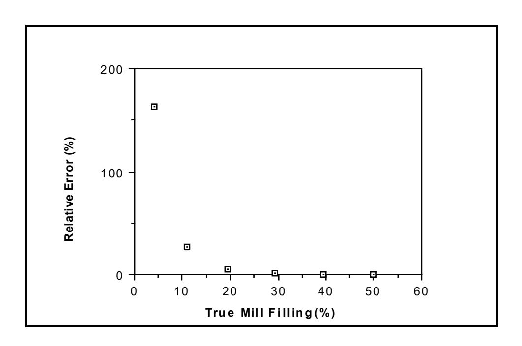
• Power Draw - plants vary widely in the type and complexity of their instrumentation. As a result power draw data were available from a range of devices including kWh meters, power transducers and ammeters. Where more than one source of power data was available at a particular site it was ensured that all sources gave similar readings. Where they did not, plant electrical staff were requested to investigate and correct the differences. Where this could not be done, the data were not included in the data base. Where only one source of power measurement was available efforts were made to ensure that independent checks of the power reading accuracy had been made either prior to the field study or shortly afterwards.
It was not possible to determine the power measurement errors within the data base. Given that considerable efforts were made in ensuring power measurement equipment was functioning properly and the rejection of some data due to conflicting measurements from different sources within plants, it is believed that the maximum error in the power measurements was less than 10%.
6.4 DATA BASE DETAILS
6.4.1 Summary
A total of 76 data sets were accumulated by the author to test the validity of the model. Details of the range of tumbling mills covered in the data base are given in Table 6.1. Full details of mill dimensions, speed, filling etc are given in Tables 6.2 - 6.4.
| Ball Mills | SAG Mills | AG Mills | |
|---|---|---|---|
| Diameter (m) | 0.85-5.34 | 1.80-9.59 | 1.8-9.50 |
| Belly Length Inside Liners (m) | 1.52-8.84 | 0.59-7.95 | 0.59-5.18 |
| Length/Diameter Ratio | 1.00-1.83 | 0.33-1.50 | 0.33-1.0 |
| Percent of Critical Speed (%) | 60-83 | 48-89 | 72-75 |
| Ball Filling (Vol %) | 20-48 | 3-25 | 0 |
| Total Filling (Vol %) | 20-48 | 7-38 | 10-31 |
| Specific Gravity of Ore | 2.6-4.6 | 2.6-4.1 | 2.7-4.6 |
| Number of Mills | 38 | 20 | 5 |
| Number of Data Sets | 41 | 28 | 7 |
| Power Draw (KW) | 6.8-4100 | 14.8-7900 | 12.5-5500 |
Of the 76 data sets, 18 were collected in person by the author in the course of fieldwork studies; 30 were collected by students/staff of the JKMRC under the author's direction; 7 were obtained from archives at the JKMRC relating to fieldwork of past staff/students, and a further 21 data sets were donated by companies sponsoring the research programmes of the JKMRC, or via studies conducted by the JKMRC's commercial arm - JKTech. Apart from the 7 historic data sets all the data were collected between the period 1988 - 1992.
6.4.2 Ball Mills
Data were collected from 38 different mills yielding a total of 41 data sets (Table 6.2). The power range of these data varied from 6.8kW to 4100kW with a corresponding diameter range of 0.85 - 5.34m. The majority of mills were of the overflow type with only 3 relatively small mills in the power range 97 - 420 kW being grate discharge.
The speed range of the mills covered by the data base ranged from 60 - 83% of critical. However the majority were in the range 70 - 75% of critical. This concentration is reflected in the speed standard deviation which at 5% is only 7% of the mean value of 73%.
Mill fillings were typically in the range 30 - 40%, though values as high as 48% and as low as 20% were recorded. Apart from one pilot mill data set, most of the low mill filling data is associated with very large diameter mills in the +4.8m range.
6.4.3 SAG Mills
SAG mill data sets numbered 28 and were associated with 20 different mills. Diameters varied from 1.8m to 9.59m with a corresponding power draw range of 15 - 7900kW. The large diameter unit also had one of the largest ball loads in the data base at 19%. Typically, however, ball loads varied in the range 10 - 15% with the mean value being 12.4%.
The speed range of the SAG mills varied from as low as 48% up to 89% of critical, with a mean of 76%. The low speed mill was fitted with a variable speed drive and was operated at this low speed specifically to generate data for the research programme. The high speed mill was from a South African gold plant.
Included in the SAG mill data base were 4 mills for which both the ore and ball charge masses were measured by dumping their contents and weighing them. Two of the mills, a 5.08 x 6.82m and a 7.05 x 3.45m unit, were dumped and analysed by the author. A third mill, a 1.8m diameter pilot unit was analysed by Mutambo (1992) and the fourth mill, a 4.16 x 4.78m machine from the Union Corporation plant in South Africa, was analysed by Mr R Pendreigh who kindly provided the author with the details.
| Discharge | Diameter | Length | Length | Length/ | Mill | Mill | Ball | Total | Ore | Gross |
|---|---|---|---|---|---|---|---|---|---|---|
| Mechanism | Inside | (Belly) | (C/line) | Diameter | Speed | Speed | Filling | Filling | sg | Power |
| Liners(m) | (m) | (m) | Ratio | (fr.crit) | (rpm) | (%) | (%) | (kW) | ||
| Overflow | 4.41 | 6.10 | 6.10 | 1.38 | 0.74 | 14.86 | 35 | 35 | 4.10 | 1900.00 |
| Overflow | 2.30 | 4.20 | 4.20 | 1.83 | 0.82 | 22.87 | 36 | 36 | 2.70 | 299.00 |
| Overflow | 2.65 | 3.40 | 3.40 | 1.28 | 0.77 | 20.08 | 36 | 36 | 2.70 | 334.00 |
| Overflow | 2.52 | 3.66 | 3.66 | 1.45 | 0.67 | 17.98 | 35 | 35 | 2.70 | 265.00 |
| Grate | 1.73 | 2.44 | 2.44 | 1.41 | 0.68 | 22.03 | 35 | 35 | 2.70 | 97.00 |
| Overflow | 3.48 | 4.62 | 4.62 | 1.33 | 0.71 | 16.10 | 39 | 39 | 2.70 | 834.00 |
| Overflow | 3.54 | 4.88 | 4.88 | 1.38 | 0.76 | 17.20 | 42 | 42 | 2.70 | 1029.00 |
| Overflow | 4.12 | 5.49 | 5.49 | 1.33 | 0.75 | 15.57 | 45 | 45 | 2.70 | 1600.00 |
| Overflow | 4.38 | 7.45 | 7.45 | 1.70 | 0.75 | 15.16 | 30 | 30 | 2.70 | 2026.00 |
| Overflow | 5.29 | 7.32 | 7.32 | 1.38 | 0.70 | 12.87 | 40 | 40 | 3.20 | 3828.00 |
| Overflow | 4.80 | 6.10 | 6.10 | 1.27 | 0.69 | 13.32 | 40 | 40 | 3.00 | 2498.00 |
| Overflow | 3.05 | 4.27 | 4.27 | 1.40 | 0.70 | 16.95 | 40 | 40 | 4.50 | 580.00 |
| Overflow | 2.60 | 3.70 | 3.70 | 1.42 | 0.69 | 18.10 | 40 | 40 | 4.50 | 347.00 |
| Overflow | 3.05 | 4.27 | 4.27 | 1.40 | 0.73 | 17.68 | 45 | 45 | 3.90 | 600.00 |
| Overflow | 3.50 | 4.42 | 4.42 | 1.26 | 0.74 | 16.73 | 35 | 35 | 2.75 | 820.00 |
| Overflow | 4.87 | 8.84 | 8.84 | 1.82 | 0.72 | 13.80 | 27 | 27 | 2.60 | 2900.00 |
| Overflow | 4.87 | 8.84 | 8.84 | 1.82 | 0.75 | 14.37 | 30 | 30 | 2.60 | 3225.00 |
| Overflow | 4.87 | 8.80 | 8.80 | 1.81 | 0.75 | 14.37 | 31 | 31 | 2.60 | 3104.00 |
| Overflow | 5.33 | 8.54 | 8.54 | 1.60 | 0.72 | 13.23 | 34 | 34 | 2.60 | 4100.00 |
| Overflow | 3.04 | 3.05 | 3.05 | 1.00 | 0.82 | 19.77 | 45 | 45 | 3.50 | 475.00 |
| Overflow | 2.29 | 2.74 | 2.74 | 1.20 | 0.83 | 23.11 | 44 | 44 | 3.50 | 235.00 |
| Grate | 1.70 | 2.70 | 2.70 | 1.59 | 0.81 | 26.27 | 40 | 40 | 2.70 | 103.00 |
| Overflow | 3.55 | 4.87 | 4.87 | 1.37 | 0.72 | 16.16 | 40 | 40 | 2.80 | 970.00 |
| Overflow | 3.50 | 4.75 | 4.75 | 1.36 | 0.75 | 16.95 | 42 | 42 | 2.80 | 921.00 |
| Overflow | 0.85 | 1.52 | 1.52 | 1.79 | 0.71 | 32.57 | 40 | 40 | 2.90 | 10.00 |
| Overflow | 0.85 | 1.52 | 1.52 | 1.79 | 0.71 | 32.57 | 20 | 20 | 2.90 | 6.80 |
| Overflow | 4.75 | 6.26 | 6.26 | 1.32 | 0.77 | 14.94 | 28 | 28 | 2.68 | 2050.00 |
| Overflow | 3.85 | 5.90 | 5.90 | 1.53 | 0.77 | 16.60 | 30 | 30 | 2.80 | 1300.00 |
| Grate | 2.64 | 3.66 | 3.66 | 1.39 | 0.70 | 18.22 | 43 | 43 | 2.80 | 420.00 |
| Overflow | 4.12 | 7.04 | 7.04 | 1.71 | 0.70 | 14.69 | 38 | 38 | 2.60 | 1800.00 |
| Overflow | 4.10 | 5.92 | 5.92 | 1.44 | 0.75 | 15.67 | 34 | 34 | 3.10 | 1525.00 |
| Overflow | 4.35 | 6.56 | 6.56 | 1.51 | 0.70 | 14.19 | 40 | 40 | 2.72 | 1850.00 |
| Overflow | 3.48 | 6.33 | 6.33 | 1.82 | 0.75 | 17.00 | 34 | 34 | 2.70 | 1150.00 |
| Overflow | 3.83 | 4.83 | 4.88 | 1.26 | 0.61 | 13.29 | 31 | 31 | 2.60 | 842.00 |
| Overflow | 4.68 | 5.64 | 5.64 | 1.21 | 0.72 | 14.08 | 48 | 48 | 2.80 | 2300.00 |
| Overflow | 4.73 | 7.01 | 7.01 | 1.48 | 0.60 | 11.76 | 32 | 32 | 2.80 | 1840.00 |
| Overflow | 5.34 | 8.69 | 8.69 | 1.63 | 0.73 | 13.36 | 28 | 28 | 3.20 | 3669.00 |
| Overflow | 5.34 | 8.69 | 8.69 | 1.63 | 0.73 | 13.36 | 26 | 26 | 3.20 | 3549.00 |
| Overflow | 5.34 | 8.69 | 8.69 | 1.63 | 0.73 | 13.36 | 24 | 24 | 3.20 | 3385.00 |
| Overflow | 5.34 | 8.69 | 8.69 | 1.63 | 0.73 | 13.36 | 23 | 23 | 3.20 | 3251.00 |
| Overflow | 3.87 | 6.34 | 6.34 | 1.64 | 0.69 | 14.83 | 27 | 27 | 4.60 | 1075.00 |
| number | 41 | 41 | 41 | 41 | 41 | 41 | 41 | 41 | 41 | 41 |
| mean | 3.73 | 5.58 | 5.58 | 1.49 | 0.73 | 17.06 | 35.25 | 35.32 | 3.03 | 1539.34 |
| sd | 1.23 | 2.15 | 2.15 | 0.21 | 0.05 | 4.73 | 6.79 | 6.80 | 0.55 | 1223.53 |
| min | 0.85 | 1.52 | 1.52 | 1.00 | 0.60 | 11.76 | 20 | 20 | 2.60 | 6.80 |
| max | 5.34 | 8.84 | 8.84 | 1.83 | 0.83 | 32.57 | 48 | 48 | 4.60 | 4100.00 |
| Dis |
Dia
meter |
Length | Length | Length/ | Mill | Mill | Ball | Total | Ore | Gross |
|---|---|---|---|---|---|---|---|---|---|---|
|
charg
e |
Inside | (Belly) | (C/line) | Diameter | Speed | Speed | Filling | Filling | Power | |
| Mech | Liners | |||||||||
| anism | ||||||||||
| (m) | (m) | (m) | Ratio | (fr.crit) | (rpm) | (%) | (%) | sg | (kW) | |
| grate | 7.73 | 3.46 | 3.46 | 0.45 | 0.70 | 10.65 | 11 | 11 | 2.60 | 1800.00 |
| grate | 6.50 | 2.42 | 3.02 | 0.37 | 0.75 | 12.44 | 6 | 21 | 3.64 | 1228.00 |
| grate | 4.35 | 4.85 | 4.85 | 1.11 | 0.75 | 15.29 | 12 | 29 | 2.60 | 1045.00 |
| grate | 7.05 | 3.45 | 3.45 | 0.49 | 0.72 | 11.47 | 12 | 33 | 2.65 | 2239.00 |
| grate | 7.05 | 3.45 | 3.45 | 0.49 | 0.72 | 11.47 | 12 | 12 | 2.65 | 1500.00 |
| grate | 5.30 | 7.95 | 7.95 | 1.50 | 0.71 | 13.04 | 18 | 30 | 2.80 | 3284.00 |
| grate | 4.05 | 4.60 | 4.60 | 1.14 | 0.76 | 15.97 | 8 | 26 | 2.70 | 688.00 |
| grate | 4.05 | 4.60 | 4.60 | 1.14 | 0.76 | 15.97 | 7 | 7 | 2.70 | 440.00 |
| grate | 4.05 | 4.60 | 4.60 | 1.14 | 0.76 | 15.97 | 6 | 32 | 2.70 | 687.00 |
| grate | 4.05 | 4.60 | 4.60 | 1.14 | 0.76 | 15.97 | 6 | 34 | 2.70 | 706.00 |
| grate | 6.51 | 2.44 | 2.44 | 0.38 | 0.71 | 11.77 | 3 | 16 | 4.10 | 972.00 |
| grate | 1.80 | 0.59 | 0.59 | 0.33 | 0.75 | 23.55 | 6 | 27 | 2.74 | 14.80 |
| grate | 9.59 | 4.27 | 5.86 | 0.45 | 0.75 | 10.24 | 14 | 14 | 2.60 | 5790.00 |
| grate | 9.59 | 4.27 | 5.86 | 0.45 | 0.75 | 10.24 | 19 | 31 | 2.60 | 7900.00 |
| grate | 9.59 | 4.27 | 5.86 | 0.45 | 0.75 | 10.24 | 17 | 30 | 2.60 | 7100.00 |
| grate | 8.39 | 3.26 | 5.00 | 0.39 | 0.80 | 11.69 | 14 | 18 | 2.68 | 4000.00 |
| grate | 4.12 | 5.02 | 5.02 | 1.22 | 0.75 | 15.63 | 22 | 22 | 2.70 | 1012.00 |
| grate | 4.12 | 5.02 | 5.02 | 1.22 | 0.75 | 15.63 | 22 | 33 | 2.70 | 1225.00 |
| grate | 4.16 | 4.78 | 4.78 | 1.15 | 0.89 | 18.44 | 10 | 38 | 2.70 | 1063.00 |
| grate | 3.90 | 5.10 | 5.10 | 1.31 | 0.78 | 16.75 | 25 | 34 | 3.35 | 1175.00 |
| grate | 5.08 | 6.82 | 6.82 | 1.34 | 0.66 | 12.38 | 12 | 31 | 2.85 | 2000.00 |
| grate | 5.05 | 5.99 | 5.99 | 1.19 | 0.77 | 14.49 | 17 | 21 | 2.68 | 2035.00 |
| grate | 5.82 | 5.65 | 5.65 | 0.97 | 0.81 | 14.20 | 13 | 33 | 2.80 | 2840.00 |
| grate | 5.80 | 5.65 | 5.65 | 0.97 | 0.81 | 14.20 | 10 | 27 | 2.80 | 2600.00 |
| grate | 3.85 | 5.69 | 5.69 | 1.48 | 0.48 | 10.35 | 12 | 12 | 2.80 | 424.00 |
| grate | 7.23 | 3.00 | 3.00 | 0.42 | 0.75 | 11.80 | 11 | 16 | 2.72 | 1920.00 |
| grate | 7.09 | 2.74 | 2.74 | 0.39 | 0.75 | 11.91 | 11 | 21 | 3.10 | 1900.00 |
| grate | 6.26 | 2.50 | 2.50 | 0.40 | 0.71 | 12.00 | 5 | 21 | 2.70 | 1200.00 |
| No. | 28 | 28 | 28 | 28 | 28 | 28 | 28 | 28 | 28 | 28 |
| mean | 5.79 | 4.32 | 4.57 | 0.84 | 0.74 | 13.71 | 12.16 | 24.25 | 2.82 | 2099.49 |
| sd | 2.01 | 1.52 | 1.55 | 0.41 | 0.07 | 3.03 | 5.67 | 8.52 | 0.34 | 1946.55 |
| min | 1.80 | 0.59 | 0.59 | 0.33 | 0.48 | 10.09 | 3 | 7 | 2.60 | 14.80 |
| max | 9.59 | 7.95 | 7.95 | 1.50 | 0.89 | 23.55 | 25 | 38 | 4.10 | 7900.00 |
6.4.4 AG Mills
Autogenous mills have the fewest number within the data base (7) and reflects their less common use compared to SAG mills. Despite this, the range of diameters that were covered in the fieldwork programme matches that of the SAG mills (1.8 - 9.50m). Due to the absence of a ball charge, however, their equivalent power range was lower than that for SAG mills (12.5-5100kW). Included were 2 mills whose entire equilibrium contents were weighed and sized. One mill was a pilot unit (Mutambo, 1992) and one was a 5.105 x 5.181m unit (Stanley, 1974).
| Discharge | Diameter | Length | Length | Length/ | Mill | Mill | Total | Ore | Gross |
|---|---|---|---|---|---|---|---|---|---|
| Mechanism | Inside | (Belly) | (C/line) | Diameter | Speed | Speed | Filling | sg | Power |
| Liners(m) | (m) | (m) | Ratio | (fr.crit) | (rpm) | (%) | (kW) | ||
| grate | 7.10 | 2.43 | 3.47 | 0.34 | 0.72 | 11.43 | 10 | 3.57 | 703.00 |
| grate | 7.10 | 2.43 | 3.47 | 0.34 | 0.72 | 11.43 | 12 | 4.60 | 1009.00 |
| grate | 6.49 | 2.25 | 2.48 | 0.35 | 0.75 | 12.45 | 27 | 4.00 | 1240.00 |
| grate | 6.49 | 2.25 | 2.48 | 0.35 | 0.75 | 12.45 | 19 | 4.00 | 960.00 |
| grate | 5.11 | 5.18 | 5.18 | 1.00 | 0.73 | 13.63 | 24 | 4.20 | 1264.00 |
| grate | 1.80 | 0.59 | 0.59 | 0.33 | 0.75 | 23.55 | 25 | 2.74 | 12.50 |
| grate | 9.50 | 4.40 | 6.40 | 0.46 | 0.75 | 10.29 | 31 | 2.90 | 5490.00 |
| number | 7 | 7 | 7 | 7 | 7 | 7 | 7 | 7 | 7 |
| mean | 6.23 | 2.79 | 3.44 | 0.45 | 0.74 | 13.60 | 21.11 | 3.72 | 1525.50 |
| sd | 2.35 | 1.53 | 1.90 | 0.25 | 0.01 | 4.51 | 7.78 | 0.69 | 1799.05 |
| min | 1.80 | 0.59 | 0.59 | 0.33 | 0.72 | 10.29 | 10 | 2.74 | 12.50 |
| max | 9.50 | 5.18 | 6.40 | 1.00 | 0.75 | 23.55 | 31 | 4.60 | 5490.00 |
6.5 CONCLUSIONS
The data base of ball, SAG and AG mills which was accumulated for this thesis covered a wide range of mills with power draws in the range 6.8 - 7900 kW.
Considerable efforts were made to ensure that the data was of a high quality, particularly with regard to power draw, dimensions and mill fillings. In the latter case fillings were obtained for 6 SAG/AG mills where equilibrium contents were dumped, weighed and sized.
In total, 76 data sets were amassed to provide sufficient numbers to rigorously test the validity of the author's models, as well as compare them to established alternatives.
CHAPTER 7
MODEL CALIBRATION AND VALIDATION
The industrial mill data base described in Chapter 6 was used to calibrate the C-model by fitting its single parameter (k). A good fit to the ball, SAG and AG mill data was found using a value for k of 1.215 for all mills. From this it was inferred that the behaviour of mills with respect to power draw was the same regardless of mill type.
To determine whether the C-model offered any better predictive capability than other published models, those of Rose and Evans (1956), Austin (1990), Harris et al (1985) and Bond (1962) were also evaluated using the data base. For ball mills only, Bond's equation was found to be almost as accurate as the C-model. With Bond's equation applied to SAG/AG mills however, the C-model was found to be significantly more accurate. For both ball and SAG/AG mills the other 3 models were all very much less accurate than the C-model. The independent data of Liddell (1986) was also used to evaluate the C-models response to speed changes. Very good agreement was observed.
The data base was also used to develop a relatively simple semi-empirical equation (Emodel) based on the performance of the C-model. It was found to provide an overall performance which was only slightly less accurate than the C-model. In the course of the development of the E-model, the diameter exponent which describes the relationship between diameter and power was found to be 2.5 when applied to net power ie. gross power less no-load power. As no-load power was found to be proportional to D2.0 the gross power diameter exponent was found to vary in the range 2.33 - 2.43 depending on the filling and speed conditions. The exponents were independent of mill type.
7.1 INTRODUCTION
Without good quality comprehensive data with which to validate a model it is of little or no practical value. To ensure that the model(s) developed in this thesis have a proven ability to accurately predict the power draw of industrial mills, an extensive data base was assembled. This chapter describes the results from using this data base to calibrate and evaluate the C-model and to compare its performance with a variety of published models. A new semi-empirical model (E-model) is also described whose performance is based on that of the C-model.
7.2 MODEL CALIBRATION
It was shown in Chapter 5 that the C-model general form was:
Gross Power = No-load Power + (k * Theoretical Net Power)
where k is a correction factor for unaccounted energy losses due to sound, heat generated within the charge due to sliding friction, rock breakage due to attrition/abrasion and rotation of the grinding media.
Initially k was set to unity and the model applied to the entire data base. For each data set the relative error was calculated as follows:
Relative Error = $$ \frac{\text{observed kW - predicted kW}}{\text{observed kW}} \times 100\% $$ (7.1)
The mean relative error was then calculated for the entire data base. The value obtained was 15% and represents energy losses in the mill which are unaccounted for by the model. The correction factor, k, was then adjusted to provide a mean relative error of <0.1%. The resultant value for k was found to be 1.215 ie. energy consumed by sound, heat generated by sliding friction within the charge, attrition/abrasion breakage and media rotation, accounts on average for an additional 21.5% of theoretical net power. This compares with Harris et al's estimates of up to 20% (1985) and Rolf and Simonis' figure of over 30% (1990).
7.3 MODEL ACCURACY
7.3.1 Error Variance
After applying the correction factor of k = 1.215, the apparent precision of the Cmodel was then evaluated using the variance of the relative error resulting from application of the model to the entire data base. The results are shown in Table 7.1 together with the 95% confidence interval. It can be seen that the standard deviation was 5.4% giving rise to a 95% confidence interval of ±10.6%. Graphically the model accuracy is also illustrated in a plot of the observed and predicted power draws (Figure 7.1).
| % | |
|---|---|
|
Relative Error
- mean |
<0.1 |
| - variance | 29.2 |
| - standard deviation | 5.4 |
| 95% Confidence interval | ±10.6 |
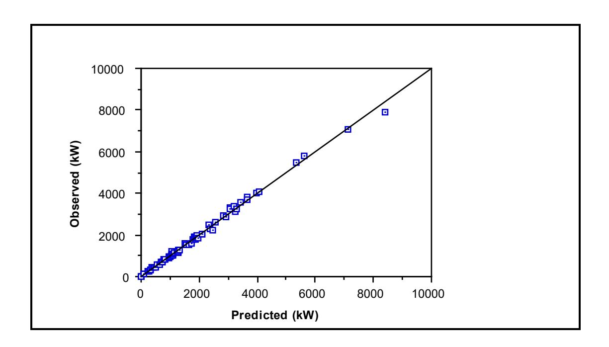
7.3.2 Contribution of Data Measurement Error
The inability of a model to match observed data can be caused by two factors:
- the model does not accurately reflect the performance of the system in question, either due to its inability to completely describe all of the system's sub-processes, or due to its omission of some of them.
- the data themselves contain measurement errors.
In practice both of the above are usually true. Thus the 5.4% standard deviation of the relative error of the C-model is a reflection of the following:
- errors in the measurements of the model input data eg. mill dimensions, mill speed, mill filling and charge density
- errors in the measurement of the actual mill power draw
- inappropriate model structure/description of physical processes which determine mill power draw
- omission of descriptions of some of the physical processes which determine mill power draw.
It might be argued that providing the data base were large and comprehensive enough then, providing the relative error variance were within certain required limits, the model could be described as being sufficiently accurate. Such an approach, however, does not differentiate between data and model accuracy and hence does not indicate the potential model performance nor the magnitude of the effects of any simplifying assumptions within the model. It was therefore decided to estimate what the likely data error contribution was.
By using estimated typical errors in the model input data (Chapter 6) a series of random errors were generated from them through the use of random number tables (Institute of Statisticians). The random error was defined as:
Random errori= Typical errori x γn (7.2)
where
Typical errori = the estimated typical measurement error for input variable i, as described in Chapter 6.
γn = n uniformly distributed random numbers.
For each data set within the data base a series of pseudo-replicate data sets were then generated by perturbing each variable in turn using these random errors. These pseudo-replicate data sets were then used as input data to the C-model.
Each of the following input variables was perturbed in turn 20 times in this fashion:
- mill diameter (D)
- mill length (L)
- fraction of mill critical speed (φ)
- mill filling (Jt)
- charge density (ρc)
- power draw
As the C-model was calibrated using the data base to provide a zero mean relative error, the application of a random error to one of the input variables resulted in the model providing a deviation of the mean relative error from zero. For each series of 20 random errors the squared mean deviations of the relative error were therefore used to calculate a variance and standard error. This variance represented the contribution of data measurement errors to the total variance. The results of this analysis are shown in Table 7.2.
| Source of Error | Variance | Standard Error (%) |
|---|---|---|
| Diameter | 6.100 | 2.47 |
| Length | 0.486 | 0.69 |
| Speed | 0.002 | 0.04 |
| Mill filling | 0.903 | 0.95 |
| Charge density | 1.823 | 1.35 |
| Power draw | 9.303 | 3.05 |
| All data | 18.607 | 4.33 |
The data relative error (standard error) amounted to 4.3%. This compares with the total standard deviation of the relative error, obtained when the C-model was applied to the data base, of 5.4%.
The difference between the values is attributed to effects such as slurry rheology, charge size distribution and lifter shape/height which are not explicitly incorporated in the model, coupled with imprecision in the models description of those processes which it does contain.
7.3.3 Model Bias
It is possible that despite a relatively low error variance some bias may exist within the model. To test this the relative errors obtained by applying the Cmodel to each data set in the data base were regressed against the data input variables to the model (Kojovic and Whiten, 1989). A significant association between one/some of the input variables would indicate an underlying bias in the model ie. the relative errors were not randomly distributed. The relative errors were regressed against the following input variables:
- diameter
- length
- speed
- charge density
- mill filling
- constant
It was found that none of the coefficients obtained from the regression was significant at the 90% level. It was therefore concluded that the errors in the model were not biased and further were not correlated with any of the input variables.
7.4 MODEL VALIDATION
Given that the model contains only one fitted parameter and that the data base is reasonably large and diverse, the fit of the model to the data as shown in the previous sections, is in itself a validation that the C-model accurately predicts the power draw of industrial grinding mills. Ideally, however, validation needs to be carried out on data independent of the data base. Although from a laboratory mill, the data obtained by Liddell (1986) presented an opportunity to validate the C-model's response to changes in mill speed and load. Liddell used a 0.545m diameter mill with a 0.308m length. It was charged with steel balls and was run at a range of speeds. For one of his series of tests the mill was charged with steel balls to a filling of 40%. A sand/water slurry of 46% solids content by volume was then added. The speed was varied in the range 50-95% of critical and the power determined using a torque meter on the motor output shaft and the mills rotational rate.
Liddell's data are shown in Figure 7.2 with the results from the C-model superimposed. The net power draw from the model is plotted as it is more likely to correspond to the measurement obtained by Liddell from his mill. This machine used a much simpler and, most likely, more efficient drive train than industrial mills against which the C-model was calibrated. In addition, the torque meter on Liddell's mill measured motor output power and hence did not include motor inefficiency. It is expected, therefore, that the net power of the C-model which is the power absorbed by the charge only, would be slightly lower than that measured by Liddell. From Figure 7.2 this is indeed the case. The C-model net power is consistently lower than that measured over the full range of speeds.
The shape of the power curve is almost identical, however, indicating a realistic response of the model to changes in mill speed.
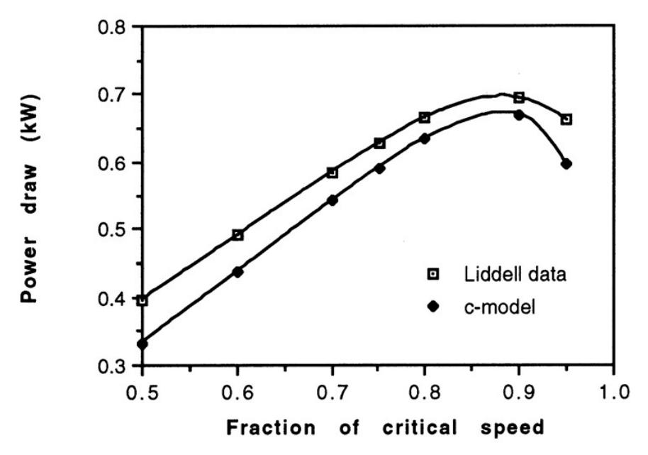
Liddell's experiments also showed that the speed at which the power draw of a mill reached a maximum was not invariant but varied with mill filling (Liddell and Moys, 1988). Figure 7.3 shows the C-model's response to speed changes for a range of mill fillings. The power draw has been normalized to provide a range of 0 - 1. It can be seen that it also predicts a maximum power draw which is dependent on filling and speed.
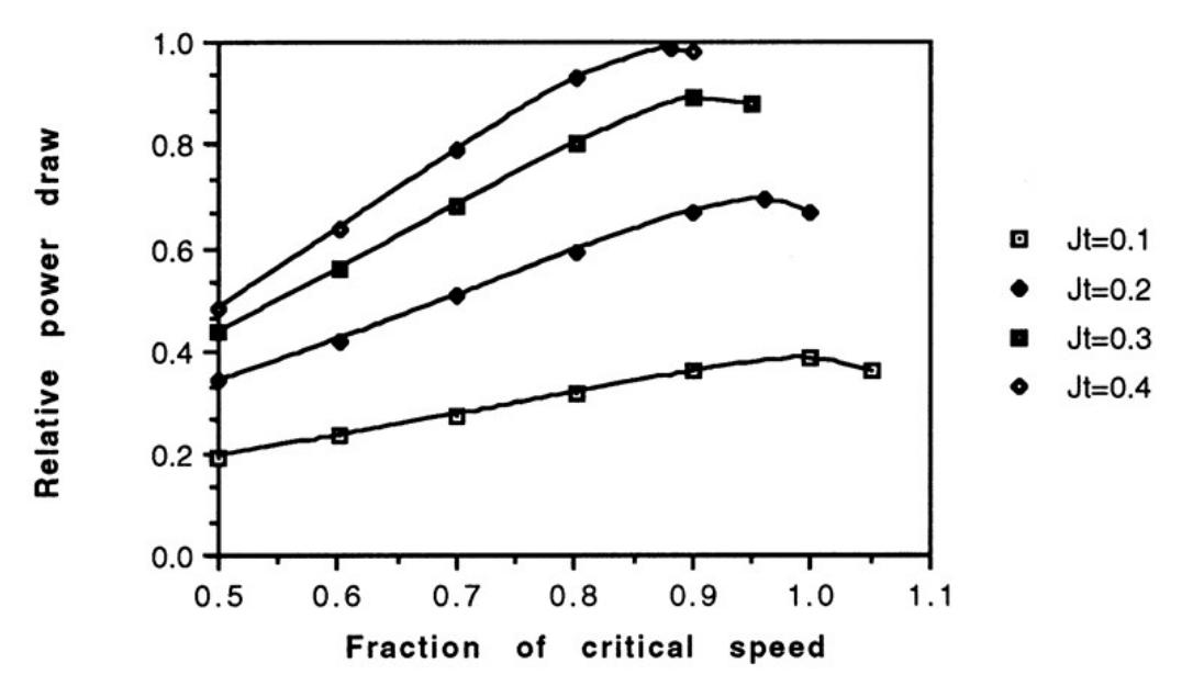
Liddell interpolated his torque data using cubic polynomials and calculated the locus of maximum torque. By multiplying the torque by the mills rotational rate he also calculated the speeds and filling at which maximum power occurred. These data are shown in Tables 7.3 and 7.4 together with the predictions using the C-model. There is reasonable agreement between Liddell's results and the Cmodel. However, from Table 7.3 the maximum fillings predicted by the C-model are slightly higher than Liddell's calculations. It should be noted, however, that the C-model indicates a very flat torque curve as Jmax is approached. Given that Liddell only had data from mill fillings at 0.3, 0.4 and 0.5, interpolating to the true maximum of the torque curve is likely to be subject to some degree of error.
| Fraction of Critical | Filling at Maximum Torque (Jmax) | ||
|---|---|---|---|
| Speed (φ) | Liddell | C-Modell | |
| .50 | 0.448 | 0.455 | |
| .60 | 0.454 | 0.492 | |
| .70 | 0.455 | 0.506 | |
| .75 | 0.463 | 0.501 | |
| .80 | 0.436 | 0.490 | |
| .90 | 0.386 | 0.412 | |
| .95 | 0.328 | 0.346 | |
| Mill Filling | Fraction of Critical Speed at Maximum Power | ||
|---|---|---|---|
| (J) | Liddell | C-Model | |
| 0.3 | >0.95 | 0.92 | |
| 0.4 | 0.88 | 0.88 | |
| 0.5 | 0.82 | 0.84 | |
7.5 COMPARISON OF C-MODEL WITH OTHER MODELS
To put the accuracy of the C-model in context, the models of Rose and Evans (1956), Bond (1962), Harris et al (1985) and Austin (1990) were also applied to the data base. Strictly speaking the models of Rose and Evans and Bond were specifically developed for ball mills whilst Austin's model was meant for SAG/AG mills. Some modifications were therefore necessary to extend the range of application of Bond's and Rose and Evan's models. Austin's model form was of a general enough nature not to require modification and was therefore applied in its original form.
7.5.1 Bond
In its revised form (Bond, 1962) Bond's equation for predicting ball mill power was given as:
kWb = $$ 3.1D^{0.3} (3.2 - 3V_p) C_s (1 - 0.1/2^{9-10C_s}) $$ (7.3)
where
kWb = mill input kW (power at pinion) per ton of grinding balls in overflow wet grinding mills
D = interior mill diameter (ft)
Vp = fraction of mill volume occupied by balls
Cs = fraction of critical speed.
For grate discharge mills kWb was multiplied by:
where
Vpd = 0.029 for wet-grinding grate and low-level discharge mills.
The above term when evaluated using \( V_{pd} = 0.029 \) gives a value of 1.1484. Converting equation 7.3 into S.I. units and using a notation consistent with the rest of this thesis gives:
Power (kW) = $$ 12.262 \rho_b \phi LD^{2.3} J_B (1 - 0.937 J_B) \left(1 - \frac{0.1}{2^{9-10\phi}}\right) $$ (7.4)
Bond's equation was meant for ball mills and hence in equation 7.4 the bulk ball density ( \( \rho_b \) ) is used ie. the contribution of the slurry fraction is not explicitly incorporated. To extend the application of the equation to SAG and AG mills \( \rho_b \) was replaced with the bulk density of the ball and/or rock charge ( \( \rho_c \) ). As with Bond's ball mill power equation the slurry fraction was not included. The charge density was therefore defined as:
$$ \rho_{c} = (1 - E) \frac{(J_{B} \rho_{b} + J_{o} \rho_{o})}{J_{t}} $$ (7.5)
where
E = grinding media voidage = 0.4
JB = fractional ball filling
Jo = fractional ore filling (excluding slurried ore)
\( J_t \) = total fractional filling = \( J_B + J_o \)
\( \rho_0 \) = ore s.g.
\( \rho_b \) = steel s.g. = 7.8.
For ball mills, equation 7.5 reduces to \( \rho_C \) = 0.6 * 7.8 which is the bulk density of the balls as per Bond's original equation. Bond's grate discharge correction was also applied to SAG and AG mills.
7.5.2 Austin
Austin developed his equation for SAG mills (Austin, 1990) and was written as follows:
where
D = mill internal diameter (m)
L = mill length (m)
Jt = fractional volume of cylindrical mill filled by total charge
JB = fractional volume of cylindrical mill filled by balls only
\( \rho_b \) = density of ball material (tonnes/m3) = 7.9 tonnes/m3
\( \rho_s \) = mean density of rock (tonnes/m3)
\( E_B \) = porosity of total charge = 0.3
\( w_c \) = weight fraction of rock in rock-plus-water in a SAG mill \( \blacktriangle \) 0.8
\( \phi_c \) = mill rotational speed as a fraction of critical speed
\( m_p \) = net mill power (power at pinion) (kW)
f3 = conical end correction.
Re-writing Austin's original correction term (f3) on the assumption that both cone ends are identical gives:
$$ f_3 = \frac{2 * 0.046}{J(1 - 1.03J)} \left\{ \left( \frac{x_1/L}{1 - D_1/2R} \right) \left[ \left( \frac{1.25 R/D}{0.5 - J} \right)^{0.1} - \left( \frac{0.5 - J_t}{1.25 R/D} \right)^{4} \right] \right\} $$ (7.7)
where
\( x_1 \) = length of the cone section (m)
\( D_1 \) = trunnion diameter (m)
R = maximum radius of cone section (m).
7.5.3 Harris et al
Harris et al's torque arm approach (1985) leads to the equation:
$$ P = 1.333\pi D^3 L \rho_c N J_t (1 - J_t) g \sin \alpha $$ (7.8)
where
P = mill power (kW) D = mill diameter (m) L = mill length (m) N = mill speed (rps) Jt = fraction of mill volume occupied by grinding media, measured at rest ρ c = bulk density of the charge (tonnes/m3).
The bulk density is calculated as follows:
$$ \rho_{c} = \frac{(J_{b} \rho_{b} + J_{o} \rho_{o})}{J_{t}} (1 - E) + E \rho_{s} $$ (7.9)
where
ρb = steel sg = 7.85
ρo = ore sg
ρs = slurry sg
Jb = fractional ball filling
Jo = fractional rock filling: Jo = Jt - Jb
E = grinding media voidage = 0.4
To determine sina, Harris et al fitted equation 7.8 to a range of manufacturer's data and obtained the following values:
Mill Type sina
Autogenous - 0.707
Overflow - 0.682 Grate - 0.809
The mill filling component of equation 7.8 was also modified to account for mills with a relatively low filling. Hence:
P = 1.33πD3 Lρ c NJt(1 - Jt)g sina ; 0.35 < Jt < 0.5
P = $$ 1.33\pi D^3 L\rho_c NJ_t(1.05 - 1.133J_t)g \sin\alpha $$ ; \( 0.2 < J_t < 0.35 \)
7.5.4 Rose and Evans
Rose and Evans (1956) used dimensional analysis to generate the following equation for predicting ball mill power draw:
where
P = power at pinion (kW)
\( \rho_s \) = steel sg = 7.9
\( \rho_p \) = slurry sg
L = mill length (m)
D = mill diameter (m)
\( N_c \) = mill critical speed (rpm)
N = actual mill speed (rpm)
Jt = fractional mill filling
h = lifter height (m)
d = ball diameter (m)
b = particle size of ore charge (m)
n = number of lifters
\( \gamma_1 - \gamma_5 \) = fitted functions.
The functions \( \gamma_1 \) - \( \gamma_5 \) were fitted to their laboratory mill data and were presented in graphical form. The functions \( \gamma_3 \) - \( \gamma_5 \) were found to be equal to unity for most conditions. The function, \( \gamma_1 \) , was approximated by them as:
where
\( \phi \) = fraction of critical speed
The function, \( \gamma_2 \) , was fitted by the author to Rose and Evans' data to give the following equation:
$$ \gamma_2 $$
(J) = 3.3506J
t
+ 1.3372 J
t
2
- 9.1602 J
t
3
(7.13)
(R
2
= 1)
The effect of the discharge type was also addressed by Rose and Evans through the application of an additional function ( \( \gamma_6 \) ) which the product of equation 7.11 was multiplied by. Once again the function was presented in graphical form. This function was also fitted by the author as follows:
$$ \gamma_6 $$
= 1.7796 - 6.2164 J
t
+ 13.6615 J
2
- 8.1923 J
3
(7.14)
(R
2
= 0.994)
Rose and Evans developed their model for ball mills and hence their charge density ( \( \rho_b \) ) is in terms of the sg of steel. To modify their equation to apply to SAG and AG mills, the \( \rho_b \) term was replaced by the mean density of the grinding media ( \( \rho_c \) ) as follows:
$$ \rho_{c} = \frac{J_{b} \rho_{b} + J_{o} \rho_{o}}{J_{t}} $$ (7.15)
where
\( \rho_0 \) = ore s.g.
Jo = volume of mill occupied by ore component of grinding media (including voids)
Jb = volume of mill occupied by ball componentof grinding media (including voids)
\( J_t \) = volume of mill occupied by total grinding charge \( (J_t = J_b + J_o) \)
For ball mills, where \( J_0 = 0 \) and \( J_b = J_t \) , equation 7.15 reduces to \( \rho_c = \rho_b \) .
7.5.5 Comparison of Model Performance
The published models used in this exercise all predict power at the output of the pinion shaft and hence do not include motor and gearbox losses. The data base and the C-model, however, all relate to motor input power. To allow for motor and gearbox losses a nominal allowances of 4% for motor losses and 3% for gearbox losses were made. Each of the models was then applied to the data base and the relative error of their predictions calculated for each data set. The mean and standard deviation of these errors was calculated for the entire data base and for the ball mill and SAG/AG mills separately. The results are shown in Table 7.5. In addition observed vs predicted power draw plots were also generated and can be seen in Figure 7.4 - 7.18.
The data show very big differences between the models. In the case of the ball mill data it can be seen that the C-model is marginally better than Bond's equation as determined by its relative error mean and standard deviation. Bond's equation tends to over predict the power draw by 2.3% though its standard deviation is only 4.7% compared to the C-model's 4.4%. The other 3 models perform quite poorly by comparison. Austin's model, as has been mentioned, was not developed for ball mills but for SAG mills. Its over prediction of the power draw of 19% and high standard deviation (9.4%) are perhaps understandable, therefore. The Rose and Evans model was developed for ball mills yet tends to under predict by 15% on average. This is in accordance with their own worked example (Rose and Evans, 1956) which, without allowance for motor and gearbox losses, predicted a power draw 23% lower than observed.
With the SAG/AG mill data the C-model is once again seen to be superior, this time by a considerable margin. Its mean relative error is 0.36% and corresponding standard deviation (6.3%). It is difficult to choose between the other models all of which have high mean relative errors and standard deviations. In fairness, however, Bond's and Rose and Evans' models were not developed for SAG/AG mills.
Overall the C-model is seen to provide both the lowest mean relative error (<0.1%) and standard deviation (5.4%). This is translated into a fairly narrow 95% confidence interval of ±10.6%. It is difficult to choose between the other models none of which, compared to the C-model, performed well. In fairness, however, their performances could be improved considerably by adjustment to their parameters so that they fitted the data base.
| Relative Error | C-model | Bond | Rose & | Austin | Harris et | |
|---|---|---|---|---|---|---|
| Evans | al | |||||
| Ball mills | - mean (%) | -0.3 | -2.3 | +15.0 | -19.2 | -27.1 |
| - sd (%) | 4.4 | 4.7 | 6.3 | 9.4 | 9.7 | |
| - 95% confidence interval (%) | 8.6 | 9.2 | 12.5 | 18.4 | 19.0 | |
| AG/SAG mills - mean (%) | +13.1 | +27.1 | -9.9 | -11.9 | ||
| - sd (%) | 6.3 | 14.7 | 9.0 | 13.8 | 11.6 | |
| - 95% confidence interval (%) | 12.3 | 28.8 | 17.6 | 27.0 | 22.7 | |
| All mills | - mean (%) | <0.1 | +5.4 | +21.0 | -14.5 | -19.5 |
| - sd (%) | 5.4 | 13.3 | 9.8 | 12.7 | 13.1 | |
| - 95% confidence interval (%) | 10.6 | 26.1 | 19.2 | 24.9 | 25.7 | |
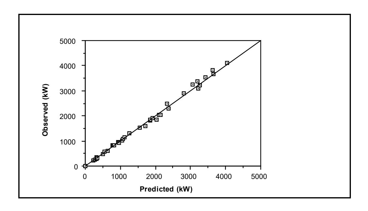
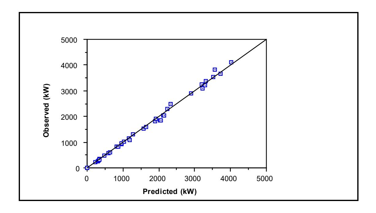
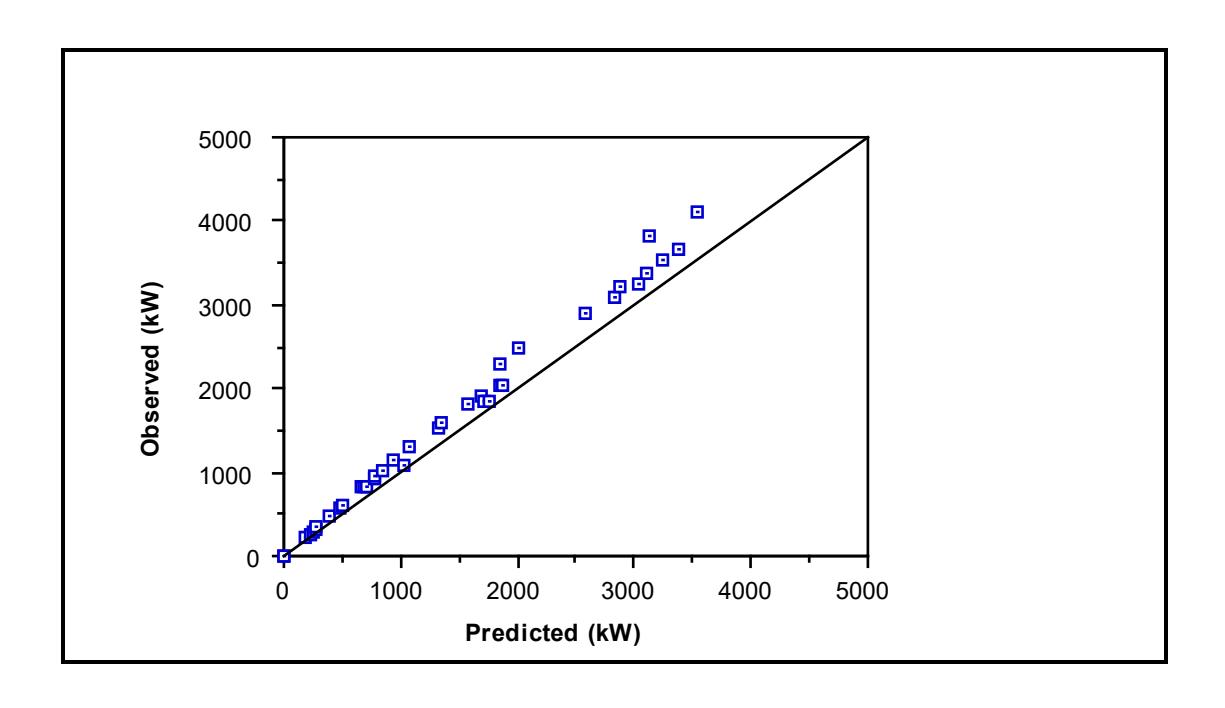
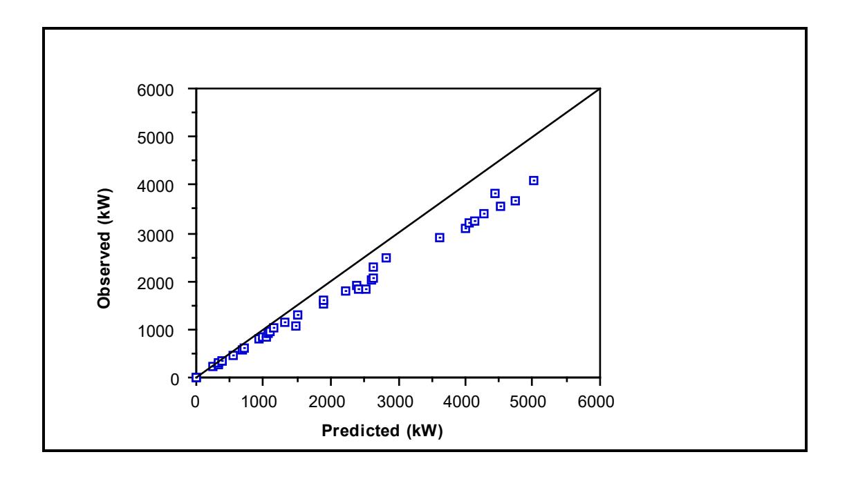
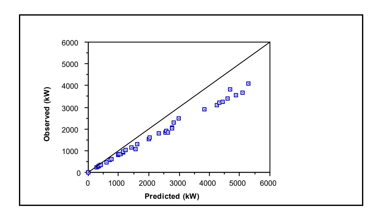
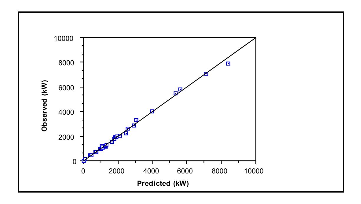
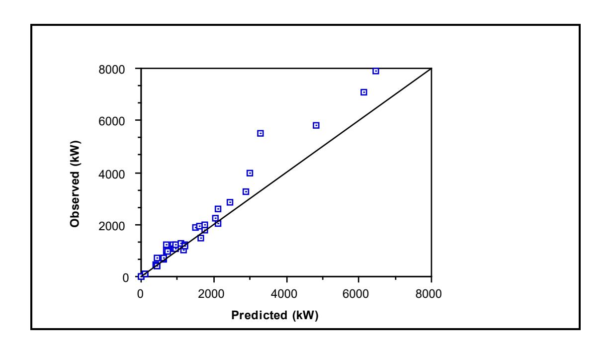
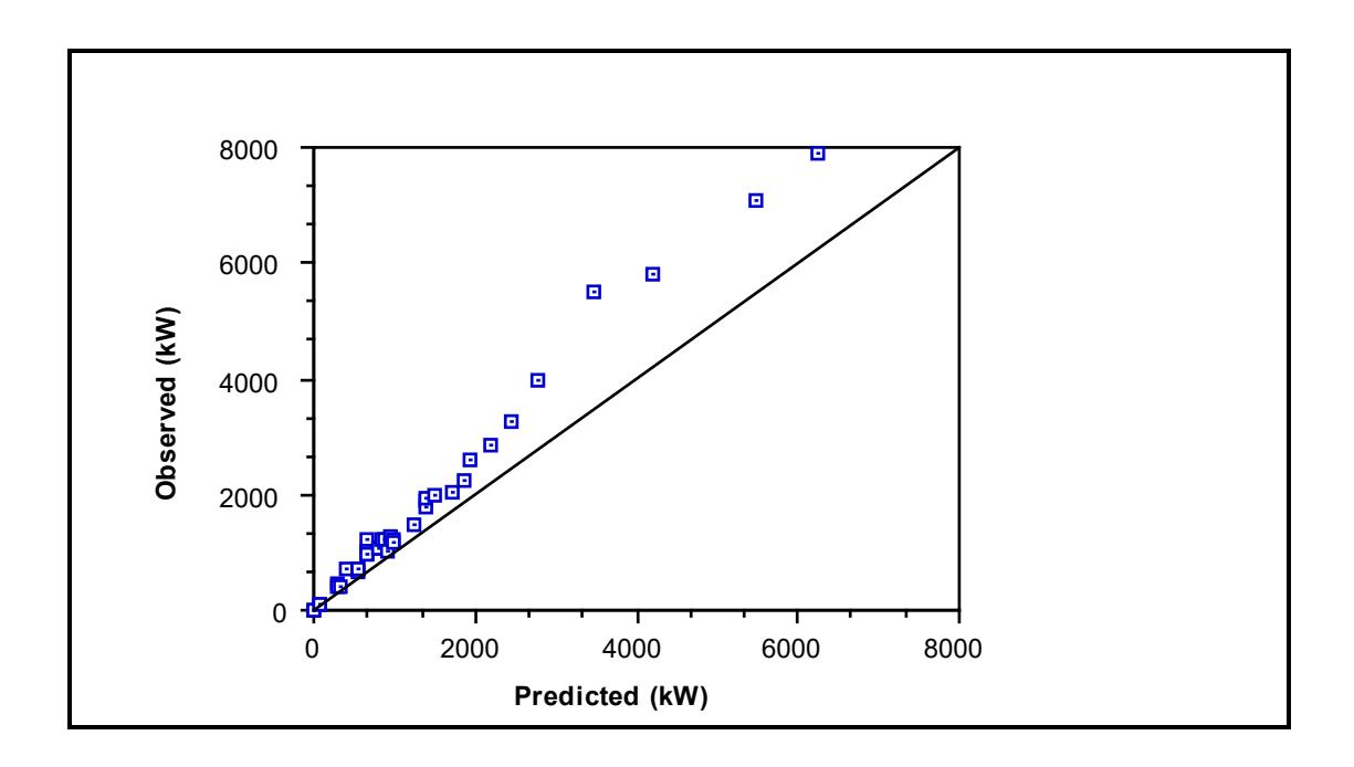
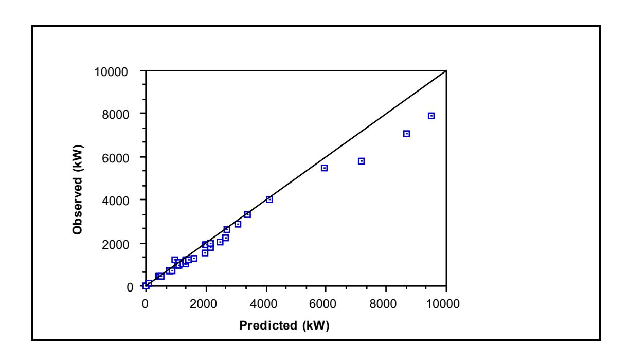
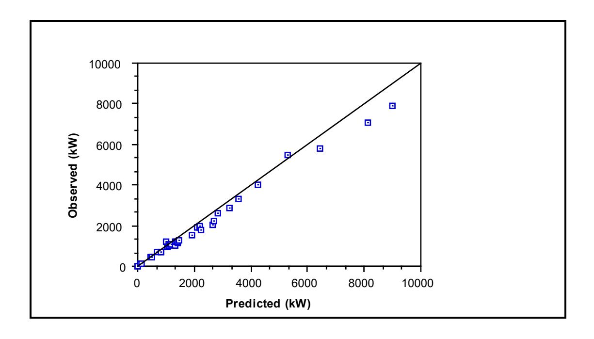
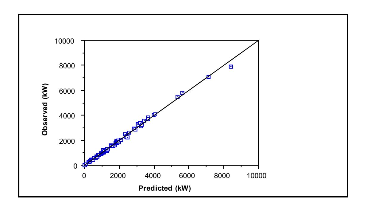
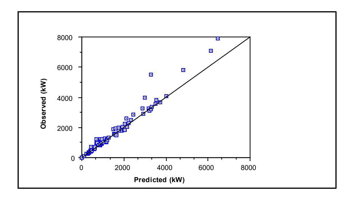
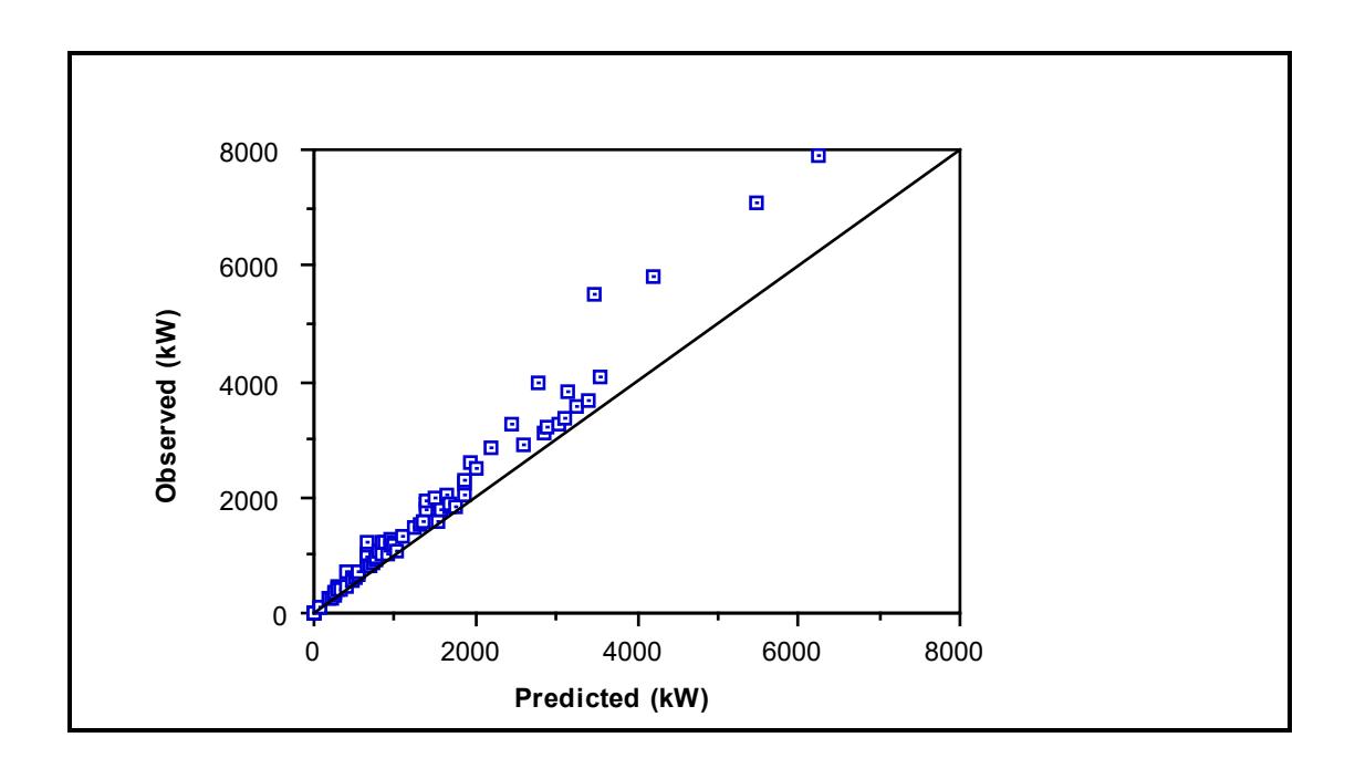
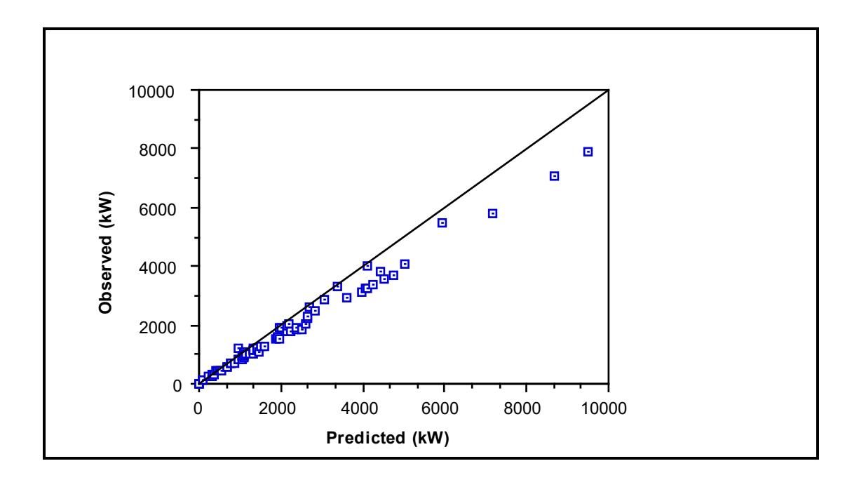
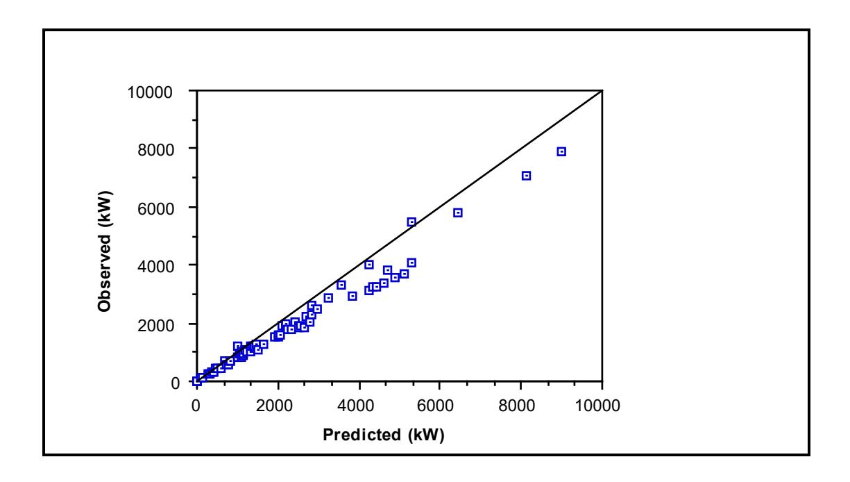
7.6 A SEMI-EMPIRICAL POWER MODEL
The availability of the data base provided an opportunity to develop a semiempirical model based on the performance of the C-model but of a much simpler form. From the analysis of the factors affecting power draw which were described in Chapters 3, 4 and 5, the following influential variables can be listed:
- diameter (D)
- length (L)
- speed (fraction of critical) (φ)
- charge density (ρc)
- mill filling (Jt)
From analysis of the C-model the relationships between these variables and power draw can be expressed simply in the form:
Net Power ∝ D2.5 Lρ c γ δ
where
γ, δ = non-linear functions of filling and speed respectively
D = mill diameter
L = mill length (effective grinding length) ρc = charge density as given by equation 5.8.
Speed and mill filling are related in a complex manner to power draw due to their influence on the toe and shoulder position. This effect is apparent in Figure 7.3 where the effect of speed changes is seen to be a function of the mill filling. Changes to mill filling at constant speed and changes to mill speed at constant filling both have the same general effect, however, ie. as mill filling and speed increase a maximum power is reached.
7.6.1 Effect of Mill Filling on Power Draw
Figure 7.19 illustrates the C-model response to changes in mill filling for a range of mill speeds. The power draw data have been normalized such that the power is in the range 0 - 1. It is seen that the filling at which power reaches a maximum (Jmax) is a function of the mill speed. The values of Jmax for the speed range 50 - 100% of critical were determined iteratively using the C-model. The results are given in Table 7.6.
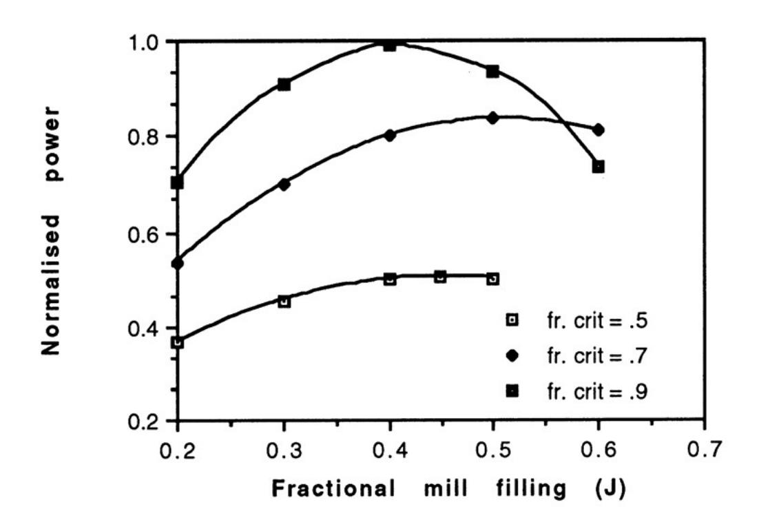
| Fraction of Critical Speed (φ) |
Filling at Maximum Net
Power (Jmax) |
|---|---|
| 0.5 | 0.455 |
| 0.6 | 0.492 |
| 0.7 | 0.506 |
| 0.75 | 0.501 |
| 0.8 | 0.490 |
| 0.9 | 0.412 |
| 0.95 | 0.346 |
| 1.0 | 0.274 |
From the data in Table 7.6 Jmax can be represented as a function of φ using the following polynomial:
From Figure 7.19 it is seen that the power draw relationship with mill filling appears to be approximately parabolic. The mill filling relationship with power can hence be expressed as:
Power $$ \propto J_t (\beta - J_t) $$ (7.17)
By differentiating power with respect to Jt and setting to zero, the filling at which power is a maximum (Jmax) can be given by:
In models such as Bond's and Austin's, β is a constant near to unity, giving an invariant power maximum at a mill filling near to 0.5 ie. Jmax ♠ 0.5. From Table 7.6 Jmax (and β) is in fact a function of mill speed. From equation 7.16 and equation 7.18, β can be represented as:
Expressing the function Jt(β - Jt) as:
then from equations 7.18 and 7.20 the maximum values of γ is :
To ensure the expression in equation 7.20 maintained values in a convenient range, regardless of mill speed, it was normalised with respect to γmax. Hence equation 7.20 was re-written as:
7.6.2 Effect of Speed on Power Draw
As with mill filling, the power draw reaches a maximum at a certain mill speed above which the power draw reduces. This effect was illustrated in Figure 7.3 where the C-model's response to mill speed was plotted. It was seen that for most of the speed range the response was approximately linear and only deviated from linear as the speed at which maximum power occurred was reached. This speed ( \( \phi_{max} \) ) is a function of the mill filling, as can be seen from Table 7.7 where values of \( J_t \) and associated values of \( \phi_{max} \) are shown. These values were obtained using the C-model. φ*max Fraction Mill Fraction of Critical Speed at Maximum Net Power (φmax) Filling (Jt) 0.9405 0.1 1.00 0.2 0.96 0.9270 0.3 0.92 0.9135 0.4 0.88 0.9000 0.5 0.84 0.8865
Table 7.7: Speed at which Power is a Maximum
To provide a speed function ( \( \delta \) ) which represented the speed trends exhibited by the C-model the following form was used:
$$ \delta = \phi \left( 1 - (1 - \phi^*_{max}) e^{-A(\phi^*_{max} - \phi)} \right) $$ (7.23)
where
A is a constant and \( \phi^*_{max} \) is related to \( \phi_{max} \)
This equation has a similar form to Bond's speed function which can be arranged as follows:
Bond speed function = $$ \phi (1 - (1 - 0.9) (2^{-10(0.9 - \phi)})) $$
Model Calibration and Validation
Not surprisingly the form of equation 7.23 is also very similar to that for describing the position of the toe (equation 3.3):
$$ \theta_{\rm T} $$ = 2.5307 (1.2796 - Jt) (1 - e -19.42 ( \( \phi_{\rm C} \) - \( \phi \) )) + \( \pi/2 \)
The exponential form of this equation results in a relatively small change in the toe angle over most of the mill speed range. At elevated speeds, however, the toe angle changes rapidly as the charge begins to centrifuge. As a result the power begins to fall. The speed function in equation 7.23 provides a similar response to speed changes. The constant (A) in equation 7.23 was therefore assumed to take the same value as in the exponential term in equation 3.3 and was set at 19.42. The parameter \( \phi^*_{max} \) was then adjusted until equation 7.23 predicted the values of \( \phi_{max} \) shown in Table 7.7. The resultant values of \( \phi^*_{max} \) are also shown in Table 7.7. They were found to be simply related to \( J_t \) by the following equation:
$$ \phi^*_{\text{max}} = 0.954 - 0.135 J_t $$ (R 2 = 1) (7.24)
7.6.3 Calibration of the Empirical Model
The empirical model (E-model) can now be written as:
Gross Power (kW) = No Load Power + (KD 2.5 L $$ \rho_c \gamma \delta $$ ) (7.25)
where: No Load Power = $$ 2.62 (D^{2.5} L \phi)^{0.804} $$ (7.26)
$$ \delta = \phi \left( 1 - (1 - \phi^*_{max}) e^{-19.42 (\phi^*_{max} - \phi)} \right) $$ (7.29)
K = calibration constant.
Due to the differences in power draw between grate and overflow discharge mills, K was fitted independently to each of these mill types in the data base. For overflow mills K was found to be 7.66 whilst for grate mills it was 8.81. The ratio of these two calibration factors is 1.15 which almost exactly matches Bond's correction factor for grate discharge mills.
7.6.4 E-Model Accuracy
The mean relative error and standard deviation of the E-model were calculated for the entire data base as well as for ball and AG/SAG mills separately. The results are shown in Table 7.8. In addition plots of observed vs predicted data are also shown in Figures 7.20 - 7.22. It can be seen that in all cases it provides very good predictive capability with only a small increase in its relative error standard deviation compared to the C-model.
| Relative Error | % | |
|---|---|---|
| Ball mills |
-
mean |
<0.1 |
|
-
sd |
5.1 | |
|
-
95% confidence interval |
10.0 | |
| AG/SAG mills |
-
mean |
<0.1 |
|
-
sd |
7.2 | |
|
-
95% confidence interval |
14.1 | |
| All mills |
-
mean |
<0.1 |
|
-
sd |
6.2 | |
|
-
95% confidence interval |
12.2 |
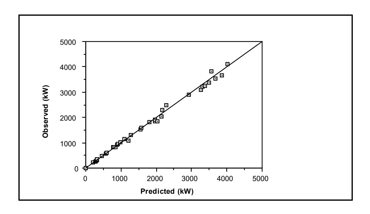
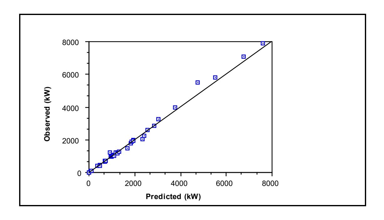
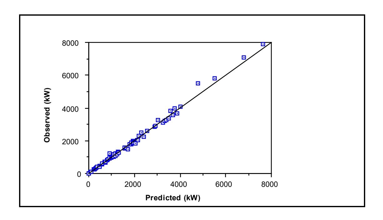
7.7 DIAMETER EXPONENT IN MILL POWER PREDICTION
It is clear from the literature that there is a conflict of opinion as to what the diameter exponent should be in grinding mill power draw equations. This is typified by the equations of Bond and Austin. Bond (1961) initially used a diameter exponent of 2.4 for ball mills but in 1962 revised it to 2.3. Austin (1990) used a value of 2.5 for AG/SAG mills based on the concensus between a number of sources (McPherson and Turner, 1978; Loveday, 1979; Dor and Bassarear, 1982). It was shown in the previous sections that the C-model fitted the data base much better than either Bond's or Austin's. It is therefore of interest to see what is the diameter exponent in the C-model. As this model is not a simple equation it is not easy to determine analytically what the exponent is. Therefore the model was used to generate a series of gross power draw data for different diameter mills under a range of conditions. The diameter exponent was then fitted to the data using simple linear regression techniques. The results are shown in Table 3. In all cases a perfect fit was obtained.
| Fraction of Critical | Mill Filling | |||
|---|---|---|---|---|
| Speed | 0.1 | 0.2 | 0.3 | 0.4 |
| 0.6 | 2.3343 | 2.3912 | 2.4118 | 2.4196 |
| 0.7 | 2.3346 | 2.3933 | 2.4150 | 2.4238 |
| 0.8 | 2.3350 | 2.3950 | 2.4172 | 2.4266 |
| 0.9 | 2.3356 | 2.3962 | 2.4185 | 2.4270 |
It is evident that the diameter exponent is not constant but over the range of conditions evaluated, varies from 2.3343 - 2.4270. The reason for this variable exponent is evident from the model structure, which divides gross power into no-load and net power:
Gross Power = No-load Power + $$ (K \times Net Power) $$ (7.31)
Empirically the no-load power was found to be related to D2 (see equation 5.24). Whereas Table 7.9 was based on gross power a similar exercise using only net power yielded a constant diameter exponent of 2.5. Hence equation 7.31 can be written as
Gross Power = $$ \alpha D^2 + \beta D^{2.5} $$ (7.32)
where
a and β relate to the other design and operating factors which affect power draw.
The mean exponent will therefore vary in the range 2 - 2.5 depending on the relative magnitude of the no-load and net power draws. Confirmation of the diameter exponent of 2.5 for the net mill power was also provided by the use of the E-model by fitting its diameter exponent rather than setting it to 2.5. The fitted exponent was 2.48 with a standard deviation of 0.018 for all mills, which agrees closely with the theoretical value of 2.5.
7.8 CONCLUSIONS
On the basis of 76 ball mill, SAG mill and AG mill data sets the C-model was found to provide accurate predictions of power draw, with a relative precision of 10.6% at the 95% confidence level. This compares with an estimated data measurement standard error of 8.5% at the 95% confidence level. Compared to the published models which were also evaluated using the same data, the C-model's performance was superior. In addition to the data base, Liddell's data (1986) from a laboratory mill run at a wide range of speeds, was also used to validate the model. Good agreement was found.
A semi-empirical model was also developed (E-model) whose response to changes in speed and mill filling was based on that of the C-model. Its predictions were found to be only marginally less precise than the C-model. Its attraction was in a more simple structure. Its equations are summarized as follows:
Gross Power (kW) = No Load Power + (KD 2.5 Lρ c $$ \gamma $$ δ)
where
No Load Power = \( 2.62 (D^{2.5} L \phi)^{0.804} \)
K = 7.66 for overflow discharge mills, and 8.81 for grate discharge mills.
Analysis of the data base and C-model response indicated that the net power draw of a mill varies as D2.5, in line with theory. Gross power, however, varies in the range D2.0 - D2.5 due to the influence of the no-load power.
CHAPTER 8
A 'DISCRETE SHELL' APPROACH TO MILL POWER MODELLING
Although it is convenient from a mathematical analysis viewpoint to consider the charge as a continuum, in practice it is particulate in nature. As a result of this charge characteristic it is found that ball/rock size has an effect on power draw (Rowland, 1972). A new model (D-model) was therefore developed to account for these effects. The model considers the mill charge to be comprised of layers or 'shells' which slide against one another. Each shell contributes to the total net power draw of the mill. The magnitude of the power draw of an individual shell is proportional to its size and velocity, both of which are functions of the charge size distribution.
The model uses similar equations to that developed for the C-model though their solution is via a computer coded algorithm rather than by analytical means. The model was calibrated using data from 4 full size and 2 pilot scale SAG/AG mills where accurate mass and size distribution data on the mill contents were known. The model was then used to predict the power draw of the 26 ball mills in the data base where make-up ball size data were known. Very good agreement was obtained. Good agreement was also obtained with Liddell's data and with Bond's predictions of ball size effects.
8.1 INTRODUCTION
In Chapter 4 the essential equations in the author's C-model were derived. To do so the charge was implicitly assumed to be continuous in nature. This is, of course, not true as the mill charge is a collection of individual rocks and/or balls. As a result the model did not consider charge particle size distribution and the effect that it may have on mill power draw. To address this deficiency and to construct a mathematical model which more closely mimics the physical conditions within a mill, a different approach was adopted. In this model (Dmodel) the charge was considered to comprise a series of discrete layers or 'shells' which slide against one another.
This chapter describes the equations and computer based algorithm which constitutes the D-model. The structure of the model, which requires a knowledge of the charge size distribution, imposed limits on the extent to which it could be calibrated and validated using the data base (detailed data on charge size distributions were only available for 6 mills). It was therefore decided to describe the D-Model in its own stand-alone chapter.
8.2 A 'SHELL' DESCRIPTION OF THE CHARGE
In Chapters 4 and 5 equations to predict the power draw of tumbling mills were developed. These were based on approximations of the patterns observed in a laboratory glass mill. The simplified charge shapes used in this model are illustrated in Figure 8.1. In developing the C-model the charge was treated as a continuum, which allowed for the analytical solution of the model equations. In reality, however, the charge is not continuous but is particulate in nature. It is more appropriate, therefore, to consider the motion of the charge as shown in Figure 8.2. In this representation the charge is assumed to comprise a series of concentric layers or 'shells'. Each shell has a mean width which is a characteristic of the size distribution of the charge. Each shell moves relative to its neighbours with the shell angular velocity decreasing the further away it is from the mill shell.
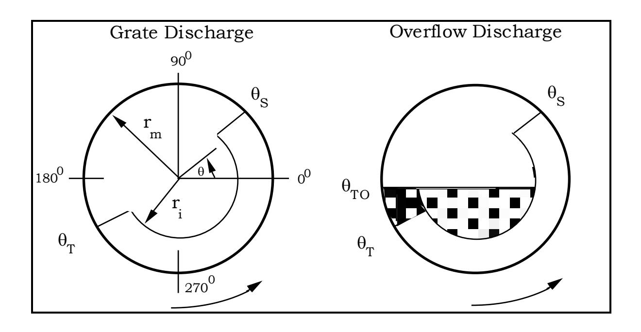
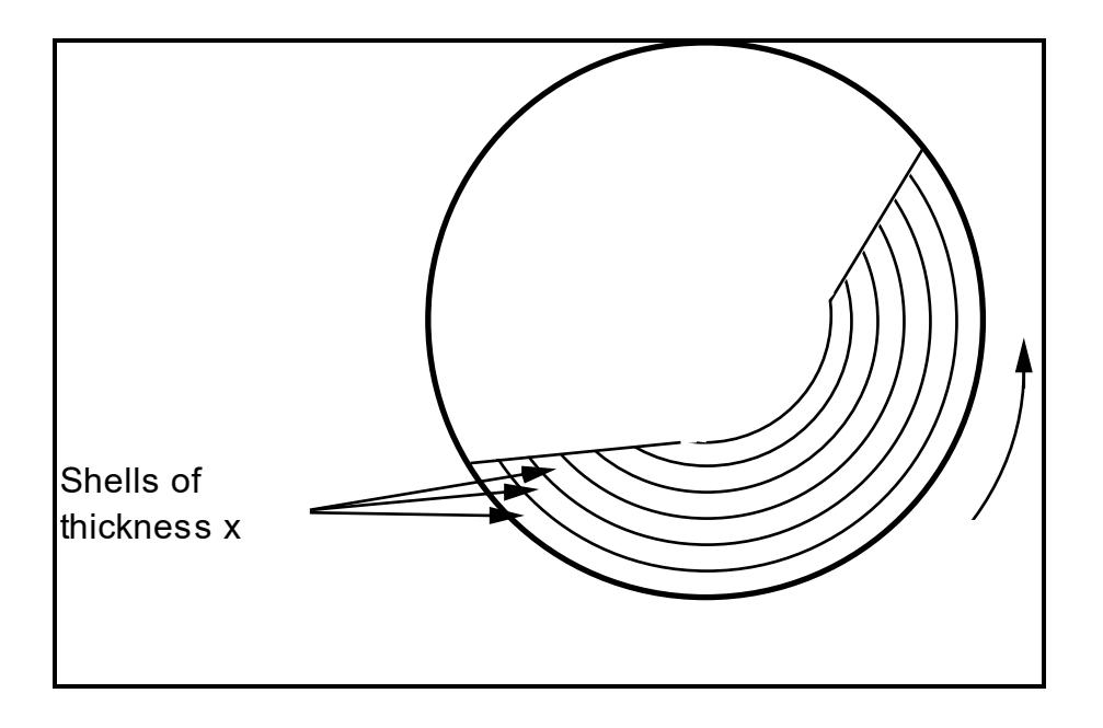
8.3 THE EFFECT OF PARTICLE SIZE
The charge in a mill is set in motion by the transfer of momentum from the mill shell. Motion is subsequently transferred throughout the charge through successive contacts between contiguous particles. As a consequence of slip between particles this mechanism results in a loss of rotational rate (rpm) from the mill shell to the centre or 'kidney' of the charge. Schematically this is illustrated in Figure 8.3.
For a given volume, a change in particle size distribution will result in a change in the number of particles and hence the number of sites at which rotational rate can be lost. A fine size distribution will therefore result in more slip within the charge, which in turn will cause a reduction in power draw.
Bond recognized this effect in his power model by introducing a factor which he used to account for what he described as 'excessive downward slippage' in larger diameter mills using make-up balls of a size less than \( \frac{1}{80} \) - \( \frac{1}{100} \) of the mill diameter (Bond, 1961/62). Bond's factor (Ss) takes the form of the following term which is subtracted from the value obtained from his power draw equation:
$$ S_{s} (kW/ton charge) = \frac{1.8 - B}{2} $$ (8.1)
where
B = ball diameter (inches)
Bond stated that the above correction was applicable to mills of 8 feet in diameter or over. Rowland (1972) added a modification to this equation for mills over 12 feet in diameter as follows:
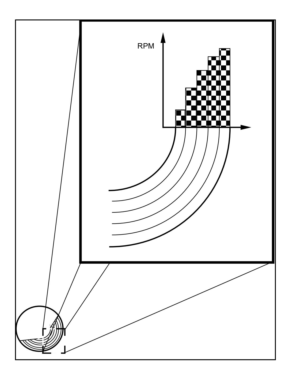
$$ S_{\rm S} = \frac{1}{40} (3D - 20B) $$ (8.2)
where
D = mill diameter (ft)
B = ball diameter (inches)
Both equations were stated to be based on plant data and studies of the charge within a glass laboratory mill. In the paper describing this work (Rowland, 1972), Rowland introduced the concept of ball layers in the mill each of which consumed different amounts of power. The connection between these layers and ball size was not made, however. Instead the loss in power associated with smaller balls was explained through an increase in the size of the inactive kidney. Rowland went on to say that a similar ball size factor existed in 'secondary autogenous (pebble) mills'. It is the authors experience that in fact the factor applies to primary autogenous and semi-autogenous mills as well. This conclusion was arrived at from observations of a number of mills where the feed size distribution coarsened and, despite the mill load mass being kept constant, the power draw increased.
8.4 SLIP WITHIN THE CHARGE AND ITS RELATIONSHIP TO FRICTION AND ATTRITION/ABRASION
The angular velocity gradient, observed within the active part of the charge, is explained by the layers of the charge slipping against one another and hence can be regarded as the 'visible' result of slip. As the layers of the charge slip in this fashion additional 'invisible' work is done in shearing the fluid layers between the grinding media, breaking rock particles between grinding media (attrition) and shearing surface particles from the grinding media (abrasion). The manifestations of these latter processes are size reduction of the rock charge, wear of the grinding media/liners and heat, either as a by-product of breakage or due to friction. The amount of slip between contiguous layers will be largely dependent on the coefficient of friction. This in turn will be related to the slurry and media surface properties such as viscosity and roughness respectively.
It might be expected, therefore, that increasing slurry viscosity would increase the coeffient of friction and, through a reduction in the amount of slip, cause an increase in power draw. In practice, however, the opposite trend is often observed ie. increasing slurry viscosity decreases power draw. Consideration of the behaviour of lubricated bearings indicates a potential resolution to this apparent anomaly.
8.4.1 Lubrication of Moving Surfaces
In 1883 Petroff described the phenomenon of friction in a bearing and shaft system using the following equation (Shigley, 1977):
$$ f = \frac{2\pi^2 \mu N r}{Pc} $$ (8.3)
where
f = coefficient of friction
µ = viscosity of the lubricant
N = rotational rate of the shaft
r = shaft radius
P = pressure exerted by the shaft on the bearing surface
c = thickness of the lubricating film.
From equation 8.3 f is proportional to µ and on the basis of this equation the mill power draw should increase with increasing viscosity. In 1932 S. A. McKee and T. R. McKee (McKee and McKee, 1932) confirmed Petroff's law but only over a proportion of the range of conditions they tested. Figure 8.4 shows their results in a plot of the bearing characteristic (µN/P) vs the coefficient of friction (f). It can be seen that Petroff's law was obeyed only in the so called thick film (stable) region. In the thin film (unstable) region Petroff's relationship was reversed and the coeffient of friction increased as viscosity decreased. In the thin film region some solid-solid contact occurred. As the viscosity decreased this tendency increased. If the plot were to be extrapolated, a point would be eventually reached where only solid-solid contact occurred. At this point the friction would be governed by the coefficient of sliding friction and would not be affected by the fluid viscosity.
Unlike a sealed bearing, within the grinding charge the lubricating slurry is free to be displaced by media approaching one another. Hence the thin film condition is more appropriate to this situation. Within this thin film region the adhesive properties of the lubricant become important. Thus as the viscosity increases the slurry tends to adhere more to the grinding media and resists being displaced as the media approach one another. This adhering layer thus promotes lubrication and slip. At the same time an increase in viscosity causes the slurry to be more entrained by the grinding media and hence is carried with it up the wall of the mill (Liddell, 1986). This effect tends to cause an increase in mill power draw. Whether an increase in viscosity will result in a decrease or increase in power draw will therefore depend on the relative magnitude of the effects of entrainment of the slurry and slip within the charge. The change in the balance between these effects is exhibited by Liddell's experiments in modifying the fluid viscosity in his laboratory mill (Figure 8.5).
It is clear from Liddell's experiments, however, that entrainment, slip and adhesion effects can interact in a complex manner and are influenced not only by viscosity but the presence of solid particles in the fluid.
8.4.2 Impact and Attrition / Abrasion Breakage
Impact breakage within grinding mills results from the grinding media falling from the shoulder region and impacting in the vicinity of the toe region. Attrition and abrasion breakage result from contiguous grinding media moving relative to one another. This type of motion will occur when the layers within the charge slip. The amount of this type of breakage will hence be affected by the number of layers and the amount of slip which occurs between them. It is to be expected, therefore, that as these factors are changed, the relative contributions of impact and attrition/abrasion of breakage will vary.
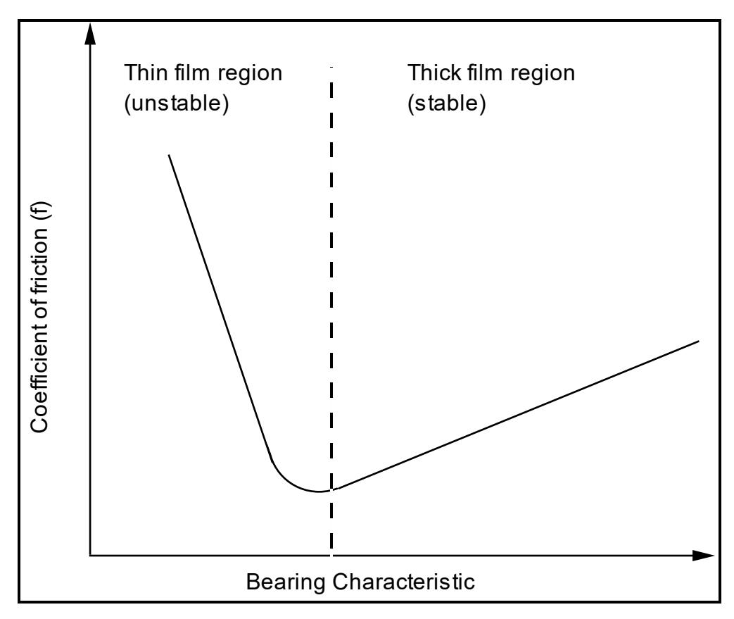
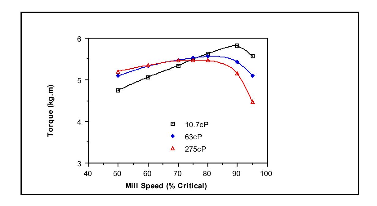
8.5 EFFECT OF LIFTERS
The effect of different lifter designs was described in Chapter 3. It was clear that different designs do change the shape of the charge. These changes, however, were relatively small and their magnitude was difficult to determine with any statistical reliability. The structures of the C and D models are designed to incorporate lifter design effects by allowing for a different relationship between the toe and shoulder angles and the mill speed and mill filling. In this work, however, a single relationship has been used which, it has been assumed, reflects the mean effect of lifter design.
From section 7 it was seen that with this assumption the C-model, when applied to the data base, resulted in a relative error standard deviation of 5.4% and a 95% confidence interval of 10.6%. It can therefore be inferred from this result that within the data base lifter effects, at most, accounted for a 10% variation in mill power. This is supported by using in the C-model the measured differences in θT and θS for the lifter types described in section 3.2. In most cases it was found that differences in θT and θS were no more than 5 and at most 10. From the C-model these differences resulted in power draw changes of approximately 5% and 10% respectively.
The effect of lifter height was not specifically examined in this work, though from Rose and Evans' research (1956) changes in lifter height are likely to account for no more than a 5% change in power draw. The effect of changing lifter height can be assumed to be simply one of preventing slip in the charge layers in direct contact with the lifters. Thus as lifter height is increased more layers of the charge will move at the same angular velocity as the mill. Using the shell concept proposed in the D-model, the effect of lifters is shown schematically in Figure 8.6 and contrasts with that shown in Figure 8.3.
8.6 A 'DISCRETE SHELL' POWER MODEL: D-MODEL
8.6.1 General Description
In the D-model the charge is divided into layers or shells, each of which has a width ( Error! ) equal to a size which is characteristic of the charge size distribution. Starting with the shell adjacent to the mill wall, the position of its toe and shoulder and its net power draw are calculated using the equation forms presented in Chapter 3 and Chapter 4. The total charge volume is then reduced by the amount associated with this shell. The process of calculating the toe, shoulder and net power draw is then repeated for the next inner shell assuming that, providing the shell is not between the tip of the lifter and the liner, slip occurs between it and the next outer shell. The process is continued for each shell until no more of the charge remains. The net power draw of the mill is calculated from the sum of the net power draws of the individual shells. The gross power draw is then calculated from the sum of the mill net power draw and no-load power as given by equation 5.24.
In the D-model, interactions between the shell width, mill speed and mill filling dictate the final shape and velocity gradient of the charge. As the charge inner surface radius cannot, therefore, be determined a priori , an iterative loop has to be used. This ensures that the number of shells, total charge volume and charge inner surface radius are all consistent.
8.6.2 Model Equations
The following sections describe the model algorithm and the equations it utilizes.
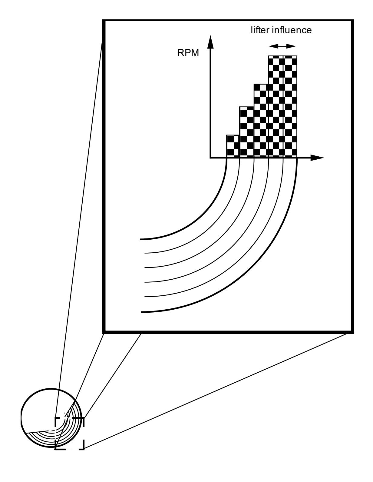
8.6.2.1 Model Algorithm
The model algorithm for calculating the net power draw is shown in Figure 8.7. The main loop within the algorithm adjusts the charge inner surface radius (ri) and hence the number of shells to be consistent with the total charge volume. In some instances it is found that with the user-given characteristic charge size ( Error! ) a value of ri consistent with the total charge volume cannot be found. A second loop is therefore incorporated in which small adjustments to Error! are also made such that a consistent value of ri can be found (the interpretation of Error! is discussed further in section 8.6.2.3).
The algorithm and equations were executed using a computer programme written in Q-Basic. A copy of the code is given in Appendix 4. Examples of the input and output screens are given in Figures 8.8 and 8.9.
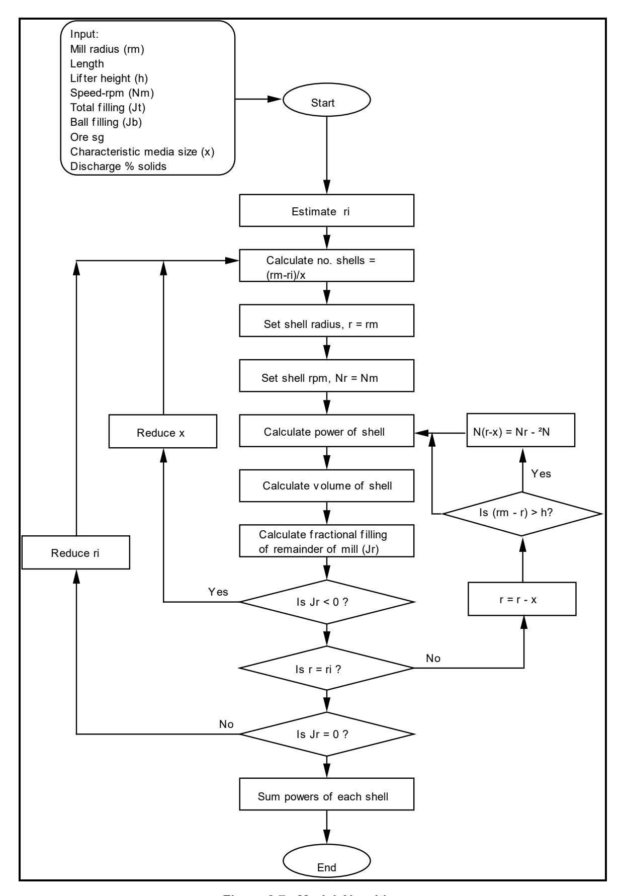
MORRELL 'DISCRETE SHELL' GRINDING MILL POWER MODEL
DIAMETER (M) 9 BELLY LENGTH (M) 4.5 C/L LENGTH 6.5 RPM10 LIFTER HEIGHT (M) .15 TRUNION DIAMETER (M) 2.6 TOTAL FILLING (%) 35 BALL FILLING (%) 10 MEAN MEDIA SIZE (M) .04 ORE SG 2.8 DISCHARGE % SOLIDS BY WT 65
IS MILL GRATE DISCHARGE (Y/N) ?Y
Figure 8.8: Example of Input Screen
| MORRELL 'DISCRETE SHELL' GRINDING MILL POWER MODEL v1.1 | |||||
|---|---|---|---|---|---|
| DIAMETER (M) | 9 | ||||
| BELLY LENGTH (M) | 4.5 | ||||
| C/L LENGTH (M) | 6.5 | ||||
| RPM | 10 | ||||
| % CRITICAL SPEED | 70.93436 | ||||
| LIFTER HEIGHT (M) | .15 | ||||
| TRUNION DIAMETER (M) | 2.6 | ||||
| TOTAL FILLING (%) | 35 | ||||
| BALL FILLING (%) | 10 | ||||
| OBS MEAN LOAD SIZE (M) | .04 | ||||
| FITTED MEAN LOAD SIZE (M) | .04 | ||||
| ORE SG | 2.8 | ||||
| DISCHARGE % SOLIDS BY WT | 65 | ||||
| GRATE DISCHARGE | |||||
| (kW) | (%) | ||||
| NET CYLINDER POWER | = | 4708.36 | 82.8 | ||
| NET CONE POWER | = | 423.72 | 7.5 | ||
| NO LOAD POWER | = | 551.45 | 9.7 | ||
| GROSS POWER | = | 5683.53 | 100 | ||
| NET IMPACT POWER | = | 3235.12 | 56.9 | ||
| NET ATTRITION/ABRASION | = | 1896.96 | 33.4 | ||
| NO LOAD POWER | = | 551.45 | 9.7 | ||
| GROSS POWER | = | 5683.53 | 100 | ||
Figure 8.9: Example of Output Screen
8.6.2.2 Loss of Rotational Rate Between Shells
It was seen in Chapter 4 that there exists an angular velocity gradient within the charge which was expressed as follows:
$$ N_{r} = \frac{N_{m}r_{m} (r - zr_{i})}{r(r_{m} - zr_{i})} $$ (8.4)
where
Assuming no slip occurs at the shell wall, then the loss of rotational rate from the shell wall to \( r_i \) is given by:
$$ N_{m} - N_{r_{i}} = N_{m} z \frac{(r_{m} - r_{i})}{(r_{m} - zr_{i})} $$ (8.5)
where
\( N_{ri} \) = rotational rate at the charge inner surface.
If the charge characteristic particle size is Error! , then it is assumed that the average shell thickness is also Error! . The number of shells (n) is therefore \( (r_m - r_i) \) / Error! and the average loss of rotational rate per shell Error! is given by:
$$ \Delta \overline{N} $$ = \( \frac{N_m z \overline{x}}{(r_m - z r_i)} \)
Equation 8.6 was generalised to provide an estimate of the loss of rotational rate between shells at radii r and \( r - \overline{x} \) as follows:
where
\( z = (1 - J_{tr})^{0.4532} \)
Jtr = fractional mill filling at a mill radius r
γ = 'slip' parameter which is expected to be related to the coefficient of friction.
To estimate a mean value for \( \gamma \) which could be used in the model, the observed angular velocity gradient from the laboratory glass mill was used to fit \( \gamma \) . This was done in an iterative manner by adjusting the value of Error! and calculating \( \gamma \) from its implicit definition in equations 8.6 and 8.7 ie.:
It was found that the velocity gradient reached a minimum when \( \gamma = 0.02433 \) at which point the model most closely approximated the observed velocity gradient. This can be seen in Figures 8.10 - 8.12 where the fit of equation 8.7 to the observed velocity gradients is shown using \( \gamma = 0.02433 \) .
As was mentioned in section 8.4, the observed velocity gradient is a result of slip within the charge. Heat generation and attrition/abrasion size reduction also occur as a result of this slip. These processes consume energy which must be supplied by the mill. In the C-model this energy was accounted for by the inclusion of a correction factor (K). In the D-model it is accounted for by adjusting the slip parameter ( \( \gamma \) )
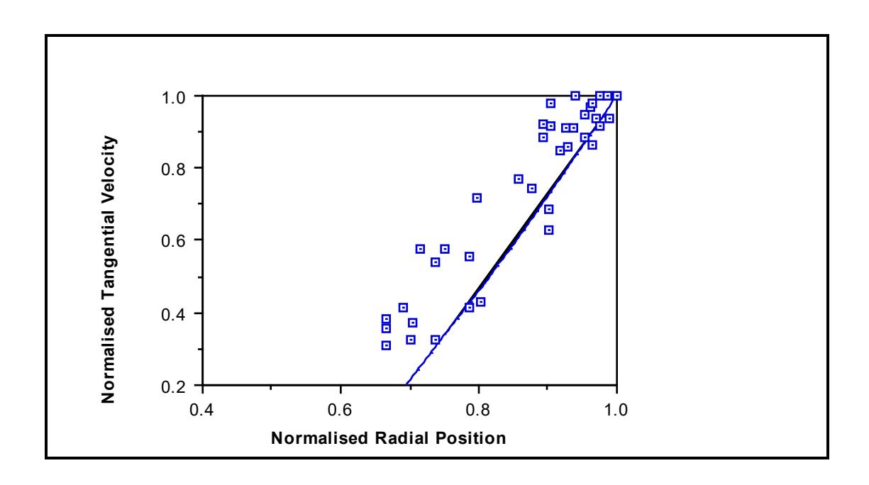
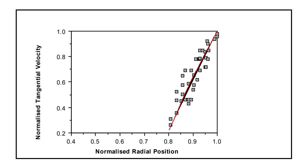
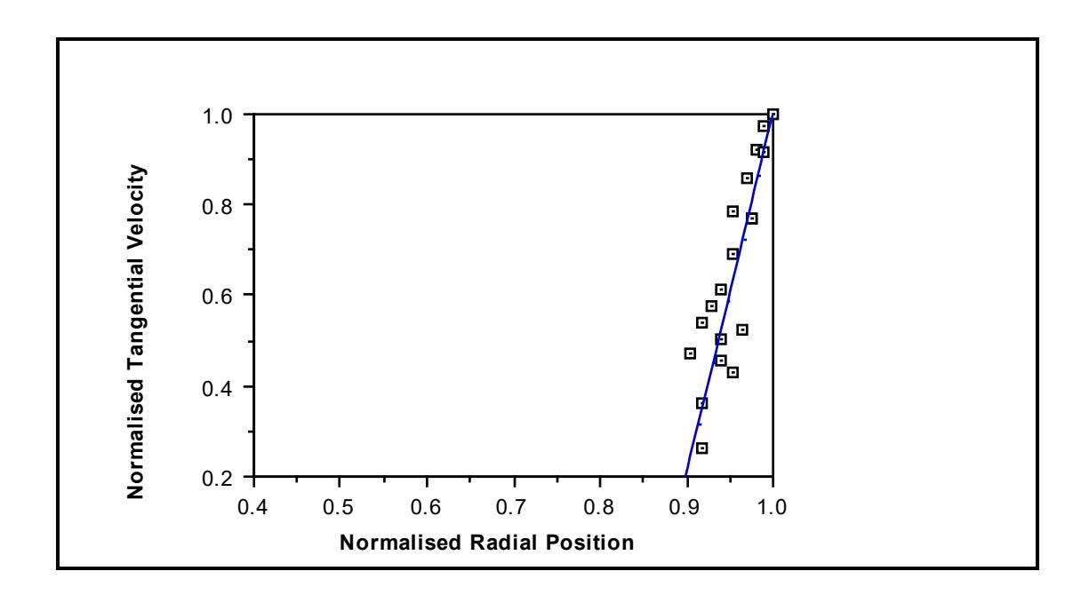
8.6.2.3 Characteristic Media Size
The thickness of shells was assumed to be a function of the particle size distribution of the charge. Thus a charge with very coarse particles will form shells which are relatively thick. The approach adopted in this model was to assume a mean thickness of shell which was related to the mean size distribution of the charge.
In a grinding mill a wide range of particle sizes will be seen. In AG/SAG mills for example the coarsest rocks may be up to 250mm whilst the smallest will be microns in size. The grinding media component of the charge will comprise the coarser rocks/balls whilst the smaller, non-media particles will fit within the interstices of the coarser fraction. It was assumed that the coarse fraction of the charge dictates the characteristic media size. It was necessary, therefore, to impose a lower size limit which defined the smallest media particle. It was assumed that this limit was related to the interstice size in the grinding charge.
If it is assumed that the media forms itself into a close-packed hexagonal structure (Figure 8.13) the diameter of particle which just slides through into the interstices is given by:
Interstice diameter = $$ D_B \left( \frac{1}{\cos 30\Box} - 1 \right) $$ (8.9)
\( = 0.15D_{B} \)
where
\( D_B \) = media diameter.
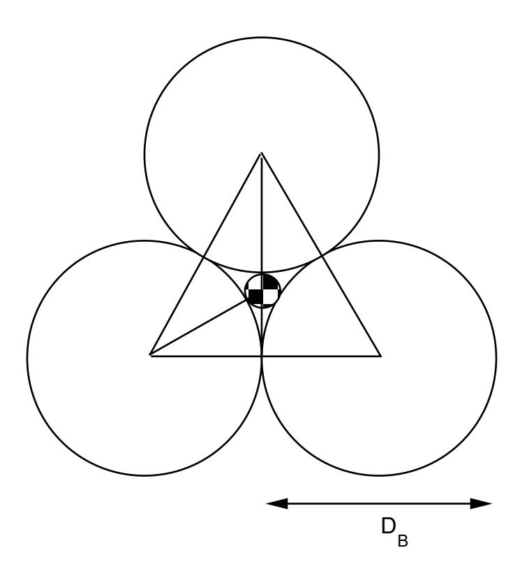
The media size distribution lower limit was therefore expected to be approximated by the following relationship:
Media size lower limit $$ \approx 0.15 \text{ M} $$ (8.10)
where
M = particle diameter characteristic of the coarsest size fraction.
The mean particle size was then defined on the basis of the grinding media size limits. As the D-model is based on the concept of slip due to particle - particle contact the mean size was based on particle numbers. Thus the mean size (Error!) was defined as:
$$ \bar{x} = \frac{\sum_{i=1}^{j} n_i x_i}{\sum_{i=1}^{j} n_i} $$ (8.11)
where
\( n_i \) = number of particles in \( \sqrt{2} \) size interval i; i = 1, 2, 3 ... j; where i = 1 is the coarsest size fraction and j is the size fraction whose geometric mean size is the media size lower
\( W_i \) = mass of particles in size interval i
\( x_i \) = geometric mean size of interval i
To determine the lower size limit of the media charge, data from the laboratory glass mill were used. From the previous section the parameter \( \gamma \) was fitted to the laboratory mill data and found to 0.02433. As the mill radius was 150mm, then from equation 8.8, Error!= 3.65mm. From the size distribution of the laboratory mill charge (Table 3.1) and equation 8.11 the lower size limit of the media charge was therefore calculated to be 1.78mm. Based on the laboratory mill charge size distribution, equation 8.10 can now be written as:
Media size lower limit (mm) = $$ 0.133 * M_1 $$ (8.12a)
or
Media size lower limit (mm) = $$ 0.165 * M_2 $$ (8.12b)
where
M1 = geometric mean of the top 2 size fraction (mm)
M2 = P95 (mm)
Both equations 8.12a and 8.12b give the same answer for the laboratory mill charge. Equation 8.12a should be used with ball mills where the top size ie. makeup ball diameter, is well defined. Equation 8.12b is more suited to SAG/AG mills where the top size is not normally well defined.
8.6.2.4 Toe and Shoulder Angles
The toe and shoulder angle equation forms developed in Chapter 3 for the Cmodel (equations 3.1 and 3.2) were also used for the D-model i.e.:
$$ \theta_{\rm T} $$ = A(1 - e -B ( \( \phi_{\rm c} \) - \( \phi \) )) + \( \pi/2 \)
$$ \theta_{S} $$ = \( \pi/2 - (\theta_{T} - \pi/2) (E + F J_{t}) \)
It was noted from experiments that centrifuging of the charge was observed as a progressive phenomenon with the outer charge layers centrifuging first. As the C and E models treated the charge as a continuum, which responded to speed changes en masse, the speed at which centrifuging occurred was taken to be when the majority of the charge was affected. Unlike the C and E models, the D-model treatment of the charge allows for the progressive onset of centrifuging. The first layer to centrifuge does so, therefore, at a lower speed than the majority of the charge. Using the D-model response to changes in mill speed, the B parameter in the toe angle equation was adjusted until the speed at maximum power in both models matched. No adjustments were made to the other parameters nor were
adjustments made to the shoulder angle equation. The resultant toe and shoulder angle equations were as follows:
$$ \theta_{\rm Tr} $$ = 2.5307 (1.2796 - J tr ) (1 - e -9( \( \phi_{\rm C} \) - \( \phi \) )) + \( \pi \) /2 (8.13)
$$ \theta_{Sr} = \pi/2 ((0.3386 + 0.1041\phi) + (1.54 - 2.5673\phi) J_{tr}) (\theta_{Tr} - \pi/2) $$ (8.14)
where
$$ \phi_{c} = \phi ; \phi > 0.35 (3.364 - J_{tr}) $$ $$ \phi_{c} = 0.3 (3.364 - J_{tr}) ; \phi \leq 0.35 (3.364 - J_{tr}) $$
where
Jtr = mill filling at radius r θTr = toe angle at radius r θSr = shoulder angle at radius r
8.6.2.5 Volume of Charge Associated with Each Shell
In order for the model algorithm to execute, the volume associated with each shell must be calculated and subtracted from the total volume of charge remaining. This was done by assuming that each shell comprised a relatively small fraction which was in flight between the shoulder and toe, and the remaining (active) portion. The active portion of the charge was calculated using simple geometry as follows:
Active charge volume = $$ 0.5 LError! $$ (8.15)
If, for a shell at radial distance r, βr is the fraction of the total shell volume accounted for by the active charge then
Total shell volume = $$ \frac{\text{Active charge volume}}{\beta_{\text{r}}} $$ (8.16)
The parameter, \( \beta_r \) , was estimated using a similar approach to that described in section 4.2.2:
where
tcr = time taken to travel between the toe and shoulder at radius r within the active portion of the shell
\( t_{fr} \) = time taken to travel in free fall between the shoulder and toe at radius r.
The times \( t_{cr} \) and \( t_{fr} \) are given by:
$$ t_{cr} = \frac{2\pi + \theta_{Sr} - \theta_{Tr}}{2\pi N_r} $$ (8.18)
$$ t_{fr} = 2r \left( \frac{\sin \theta_{Sr} - \sin \theta_{Tr}}{g} \right)^{0.5} $$ (8.19)
8.6.2.6 Power Draw Equations
In the D-model the power draw attributed to each shell is computed separately. The sum of the powers associated with each shell is therefore the power draw of the entire charge.
If a shell of width Error! is considered to be between radial positions r and r- Error! from the axis of rotation of the mill, then, on the basis of the theory developed in chapters 4 and 5, the net power associated with it \( (P_r) \) is given by:
+
$$ 4\pi^3 $$
\( \int_{-\infty}^{r} N_r^3 r^3 L\rho_c dr \)
\( r-\bar{x} \)
$$ + 2\pi \int_{r-\overline{x}}^{r} \frac{\theta_{Tr}}{\int_{r-\overline{x}}^{r}} N_r r^2 L\rho_p g \cos\theta d\theta dr $$ (8.20)
The 3 terms in equation 8.20 refer to the potential energy of the charge, the kinetic energy of the charge and the potential energy of the slurry pool. Integrating each of the terms therefore gives:
$$ P_{r} = \frac{2}{3} \pi LgN_{r}(r^{3} - (r-\bar{x})^{3}) \left( \rho_{c} \left( \sin\theta_{Sr} - \sin\theta_{Tr} \right) + \rho_{p} \left( \sin\theta_{Tr} - \sin\theta_{TO} \right) \right) + \pi^{3} L \rho_{c} N_{r}^{3} (r^{4} - (r-\bar{x})^{4}) $$ (8.21)
where
r = radial distance of the shell from the centre of rotation (m)
L = mill length of cylindrical section (m)
\( \rho_c \) = charge density (tonnes.m-3)
\( \rho_p \) = discharge pulp density (tonnes.m-3)
\( \theta_{Sr} \) = shoulder angle at radius r (rads.)
\( \theta_{Tr} \) = toe angle at radius r (rads.)
\( \theta_{TO} \) = overflow angle, \( \theta_{TO} \) = 3.395 rads for overflow mills
and \( \theta_{TO} = \theta_{Tr} \) for grate discharge mills
g = gravitational constant (m.s-2)
\( N_r \) = rotational rate at r (revs.s-1).
8.6.2.7 Conical Ends
The treatment of conical ends within the D-model is a simple extension of the algorithm for the cylindrical section. It treats the cone ends as a series of cylindrical sections each of thickness Error! and decreasing radius consistent with the geometry of the actual cone (Figure 8.14). The power of each small cylindrical section is calculated using an algorithm similar to that used for the main cylindrical section. It is assumed that the charge inner surface radius within the cone is the same as within the cylindrical section. The main loop within the cone algorithm therefore adjusts the cone charge volume to be consistent with the charge inner surface radius.
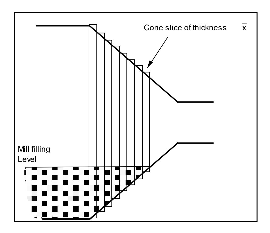
8.7 MODEL CALIBRATION
If the grinding media size distribution is known then the only unknown in the model equations is the γ parameter, which is expected to be a function of factors such as the slurry viscosity and coefficient of dynamic friction. To determine what the value of γ should be, all of the mills from the author's data base where ball/ore charge size distributions had been measured were selected. These comprised 4 SAG mills and 2 AG mills.
Using equations 8.11 and 8.12, the characteristic size of each charge was determined and the slip parameter γ adjusted until the mean relative error of the model prediction was < 0.1%. A mean value of 0.0028 for γ was obtained. The resultant fit to the 6 SAG/AG mills is shown in Figure 15. The standard deviation of the relative error was 4.23%.
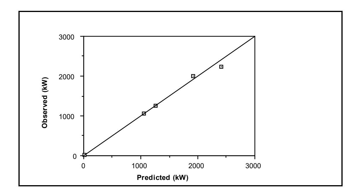
8.8 MODEL VALIDATION
8.8.1 Ball Mill Data
In SAG/AG mills a large proportion of the grinding charge is comprised of rock which varies in quantity and size distribution depending on feed ore conditions (Lynch and Morrell, 1992). Other than by simulation (Leung 1987, Morrell 1992), it is therefore not easy to determine the size distribution of SAG/AG mill charges. Hence, apart from the 6 cases used to calibrate the model, prediction of the power draw of the other SAG/AG mills in the data base was not possible.
Unlike SAG/AG mills, ball mill media charge size distributions typically follow a reasonably well defined pattern. This is due to the predictable way that most balls wear (Bond, 1943; Azzaroni, 1987). From this work it can be assumed that for practical purposes an equilibrium ball charge in a ball mill will have equal numbers of balls per unit size fraction eg. the number of balls in size fraction -50 +40mm will be equal to the number in size fraction -40 +30mm and so on. Thus if the make-up ball size is T and the smallest ball in the charge is S, then the mean size as defined by equation 8.11 is equivalent to:
From equation 8.12a, S is given by:
$$ S = 0.133 * T * 2^{-0.25} $$ (8.23)
Substituting S into equation 8.22 gives
$$ \bar{x} = 0.5559T $$ (8.24)
From the ball mill data base, 26 data sets included make-up ball size information. Using equation 8.24 to estimate Error! , and the value for \( \gamma \) of 0.0028 determined using the SAG/AG mill data, the model was used to predict the power draws of each of these ball mills.
Overall the mean relative error was found to be -2.2% indicating a slight overprediction of the power draw. To correct this, a minor adjustment was made to the overflow toe angle (θTO) which was reduced to 3.3 radians. Its effect was to slightly increase the volume of slurry in the toe region and hence reduce the power draw. This correction reduced the mean relative error to <0.2%. The standard deviation of the relative error was 3.4% giving a 95% confidence interval of 6.6%. A plot of the observed and predicted power draws are given in Figure 8.16. Full details of the mills are also given in Table 8.1 together with the predicted power draws.
| Disch. | Diam. | Length | Length | Mill | Ball | Ball | Char. | Total | Ore | Obs. | Pred. | Rel. |
|---|---|---|---|---|---|---|---|---|---|---|---|---|
| mech. | (Belly) | (C/line) | Speed | Filling | Size | Size(x) | Filling | sg |
Gross
Power |
Gross
Power |
Error | |
| (m) | (m) | (m) | (fr.cr.) | (%) | (mm) | (mm) | (%) | (kW) | (kW) | |||
| o/f | 4.41 | 6.10 | 6.10 | 0.74 | 35 | 65 | 36 | 35 | 4.10 | 1900.0 | 1894.4 | 0.003 |
| o/f | 2.30 | 4.20 | 4.20 | 0.82 | 36 | 52 | 29 | 36 | 2.70 | 299.0 | 309.8 | -0.036 |
| o/f | 2.65 | 3.40 | 3.40 | 0.77 | 36 | 65 | 36 | 36 | 2.70 | 334.0 | 335.7 | -0.005 |
| o/f | 2.52 | 3.66 | 3.66 | 0.67 | 35 | 52 | 29 | 35 | 2.70 | 265.0 | 267.9 | -0.011 |
| o/f | 3.48 | 4.62 | 4.62 | 0.71 | 39 | 56 | 31 | 39 | 2.70 | 834.0 | 817.7 | 0.020 |
| o/f | 3.54 | 4.88 | 4.88 | 0.76 | 42 | 80 | 44 | 42 | 2.70 | 1029.0 | 1027.9 | 0.001 |
| o/f | 4.12 | 5.49 | 5.49 | 0.75 | 45 | 80 | 44 | 45 | 2.70 | 1600.0 | 1668.3 | -0.043 |
| o/f | 4.38 | 7.45 | 7.45 | 0.75 | 30 | 50 | 28 | 30 | 2.85 | 2026.0 | 2090.6 | -0.032 |
| o/f | 5.29 | 7.32 | 7.32 | 0.70 | 40 | 80 | 44 | 40 | 3.20 | 3828.0 | 3557.7 | 0.071 |
| o/f | 4.87 | 8.84 | 8.84 | 0.72 | 27 | 55 | 31 | 27 | 2.60 | 2900.0 | 2862.5 | 0.013 |
| o/f | 4.87 | 8.84 | 8.84 | 0.75 | 30 | 55 | 31 | 30 | 2.60 | 3225.0 | 3201.2 | 0.007 |
| o/f | 4.87 | 8.80 | 8.80 | 0.75 | 31 | 55 | 31 | 31 | 2.60 | 3104.0 | 3187.2 | -0.027 |
| o/f | 5.33 | 8.54 | 8.54 | 0.72 | 34 | 55 | 31 | 34 | 2.60 | 4100.0 | 3960.1 | 0.034 |
| o/f | 3.55 | 4.87 | 4.87 | 0.72 | 40 | 90 | 50 | 40 | 2.80 | 970.0 | 948.0 | 0.023 |
| o/f | 3.50 | 4.75 | 4.75 | 0.75 | 42 | 58 | 32 | 42 | 2.80 | 921.0 | 944.2 | -0.025 |
| o/f | 0.85 | 1.52 | 1.52 | 0.71 | 40 | 65 | 36 | 40 | 2.90 | 10.0 | 9.4 | 0.061 |
| o/f | 0.85 | 1.52 | 1.52 | 0.71 | 20 | 65 | 36 | 20 | 2.90 | 6.8 | 6.6 | 0.029 |
| o/f | 3.85 | 5.90 | 5.90 | 0.77 | 30 | 45 | 25 | 30 | 2.80 | 1300.0 | 1244.0 | 0.043 |
| o/f | 4.12 | 7.04 | 7.04 | 0.70 | 38 | 61 | 34 | 38 | 2.60 | 1800.0 | 1831.6 | -0.018 |
| o/f | 5.34 | 8.69 | 8.69 | 0.73 | 23 | 80 | 44 | 23 | 3.20 | 3251.0 | 3221.1 | 0.009 |
| o/f | 4.73 | 7.01 | 7.01 | 0.60 | 32 | 52 | 29 | 32 | 2.80 | 1840.0 | 1887.4 | -0.026 |
| o/f | 4.10 | 5.92 | 5.92 | 0.75 | 34 | 52 | 29 | 34 | 3.10 | 1525.0 | 1529.9 | -0.003 |
| o/f | 4.35 | 6.56 | 6.56 | 0.70 | 38 | 65 | 36 | 38 | 2.72 | 1850.0 | 1928.3 | -0.042 |
| o/f | 3.48 | 6.33 | 6.33 | 0.75 | 34 | 72 | 40 | 34 | 2.70 | 1150.0 | 1121.5 | 0.025 |
| o/f | 3.87 | 6.34 | 6.34 | 0.69 | 27 | 40 | 22 | 27 | 4.60 | 1075.0 | 1129.5 | -0.051 |
| o/f | 3.83 | 4.83 | 4.88 | 0.63 | 31 | 52 | 29 | 31 | 2.60 | 842.0 | 819.7 | 0.026 |
| No. | 26 | 26 | 26 | 26 | 26 | 26 | 26 | 26 | 26 | 26 | 26 | 26 |
| Mean | 3.81 | 5.90 | 5.90 | 0.72 | 34 | 61 | 34 | 34 | 2.90 | 1614.8 | 1607.8 | 0.002 |
| S.d. | 1.22 | 2.11 | 2.11 | 0.05 | 6 | 13 | 7 | 6 | 0.48 | 1189.7 | 1160.5 | 0.033 |
| Min. | 0.85 | 1.52 | 1.52 | 0.605 | 20 | 40 | 22 | 20 | 2.6 | 6.8 | 6.6 | -0.051 |
| Max. | 5.34 | 8.84 | 8.84 | 0.82 | 45 | 90 | 50 | 45 | 4.6 | 4100.0 | 3960.1 | 0.071 |
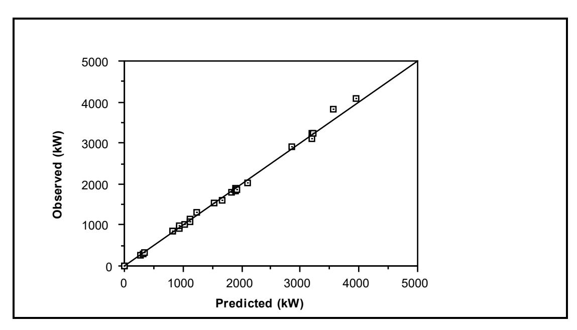
8.8.2 Effect of Changing Mill Speed
The model's response to changes in speed was also evaluated using Liddell's laboratory mill data. The results are shown in Figure 8.17 where the model's predicted net power is plotted. It is seen that it matches the measured response of Liddell's mill very well.
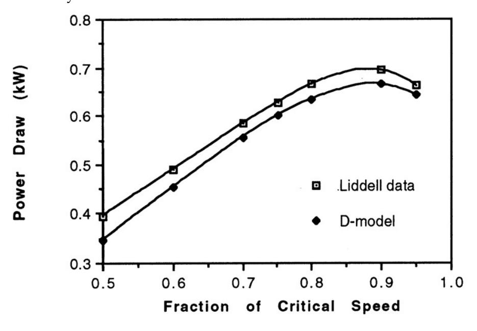
8.8.3 Ball Size Effects
The structure of the D-model specifically addresses the effect of changing ball size. Unfortunately data were not able to be collected on the observed changes in mill power due to a change in ball size. Bond's and Rowland's ball size correction factor, however, is an empirically derived equation which should reflect the changes they observed in operational mills where the ball size was changed. The D-model was therefore used to predict the power draw of a range of mill diameters and ball sizes. In each case the length was set to the same dimension as the diameter, mill speed was set at 70% of critical and the ball filling was 0.4. The results were then compared to those obtained using Bond's and Rowlands formulae (equations 8.1 and 8.2). The equations were applied according to Rowland's guidelines (Rowland, 1972) ie. Bond's equation for diameters in the range 8 - 12ft and Rowland's in the range +12ft. The results are shown in Table 8.2.
| Diameter (m) | ||||||||||
|---|---|---|---|---|---|---|---|---|---|---|
| 5 | 4 | 3 | ||||||||
|
Ball Size
(mm) |
D-Model
(kW) |
Bond
(kW) |
D-Model
(kW) |
Bond
(kW) |
D-Model
(kW) |
Bond
(kW) |
||||
| 25 | 2010 | 1979 | 966 | 973 | 371 | 378 | ||||
| 50 | 2160 | 2087 | 1016 | 1027 | 386 | 401 | ||||
| 75 | 2208 | 2194 | 1034 | 1082 | 390 | 424 | ||||
| 100 | 2231 | 2301 | 1041 | 1137 | 392 | 447 | ||||
Graphically the results are displayed in Figures 8.18 - 8.20. The linear trend of Bond's and Rowland's formulae is clearly evident. However both Bond's and Rowland's work indicated that ball size effects were only readily apparent when the ball size was less than 0.01 - 0.0125 of the mill diameter. This ball size range has been drawn in Figures 8.18 - 8.20 to indicate the point at which their correction factors should begin to be applied. The D-model, in contrast to the Bond/Rowland equation, shows a marked non-linear effect with regards to ball size. It predicts that the ball size effect reduces as the ball size increases. This point coincides very well with the empirically derived range from Bond's and Rowland's work of 0.01 - 0.0125 of the mill diameter.
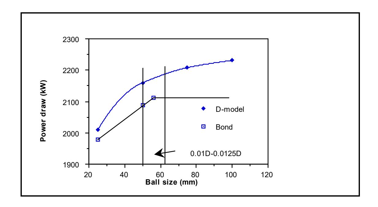
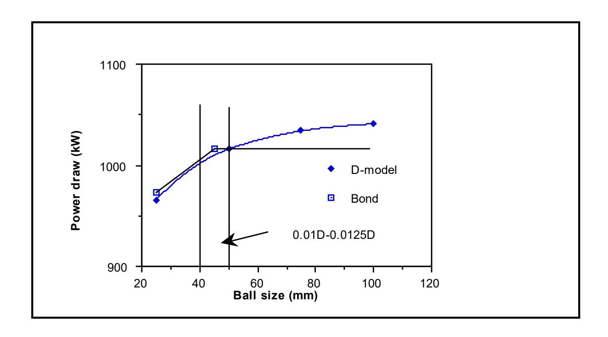
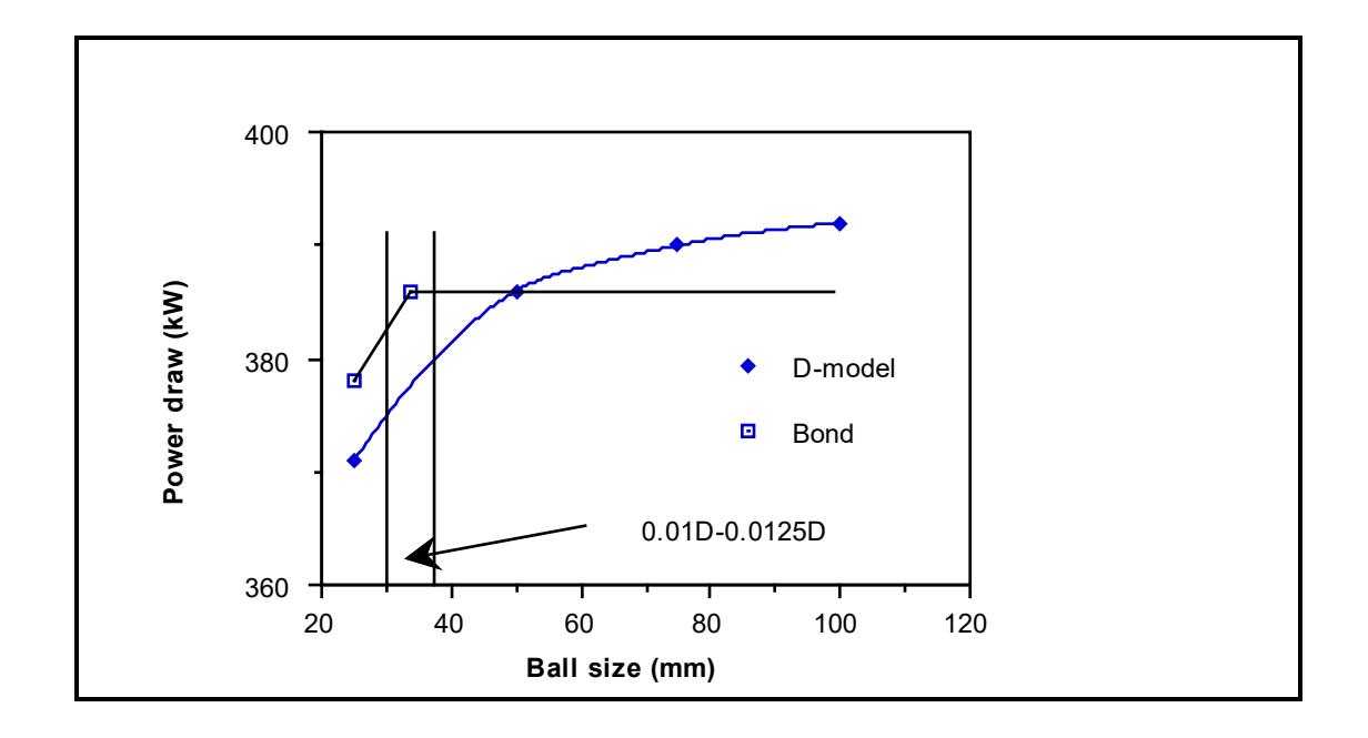
Figure 8.20: Effect of Ball Size: 3m Diameter Mill
8.9 POWER CONSUMED BY IMPACT AND ATTRITION/ABRASION
It was assumed that if no attrition/abrasion took place, and the shearing of the fluid between the media and sliding contact between media was achieved without heat loss, a different velocity gradient to that observed in the laboratory mill would result. This gradient would be less pronounced and would tend more to the no-slip condition, resulting in more lift to the charge and more impact breakage. Put another way - the generation of heat and attrition/abrasion breakage between the grinding media consume energy which results in a loss of rotational rate within the charge. The difference between the observed velocity gradient and one assuming no friction nor attrition/abrasion breakage will therefore provide an estimate of the power consumption for these processes. By using the power draw data from industrial mills, where the charge size distribution and hence Error! was available, it was possible to back-calculate the slip parameter (γ) to match the observed power draw. This was equivalent to assuming that all friction heat losses and attrition/abrasion energy was used to provide additional lift to the charge which was subsequently converted into impact breakage energy.
The value for γ which was fitted to industrial power data was 0.0028, whilst that determined using the observed velocity profile from the laboratory mill was 0.02433. The D-model was therefore run with γ set at both these values. The difference between the 2 predictions was expressed as the attrition/abrasion fraction of total power draw. This was carried out for the same range of mill diameters and conditions as was used to validate the ball size performance of the model. The results are shown graphically in Figure 8.21. It can be seen that the attrition/abrasion power fraction is a strong function of the ball size. As the ball size decreases the abrasion/attrition fraction increases. There is also an apparent diameter relationship, such that for a given ball size the attrition/abrasion fraction increases with increasing diameter. The model suggests that for a 4-fold decrease in ball size the attrition/abrasion fraction will double.
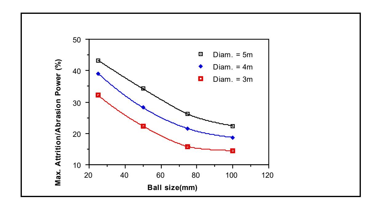
8.10 CONCLUSIONS
By considering the mill charge to comprise a series of discrete layers or shells which move with a relative angular velocity to one another, a model (D-model) was developed which successfully accounted for ball/rock size effects on power draw. The model was calibrated using SAG/AG mill data for which charge size distributions and masses were known. The model was then applied to 26 ball mill data sets where the make-up ball size only was known. By using a simple ball wear relationship the equilibrium ball size distribution was estimated and used in the model. The resultant predictions showed very good agreement with the observed power draws.
The model was used to predict the effect of grinding media size distribution on power draw. It was found to predict that as the size distribution of the grinding media became finer the power draw decreased. Increasing the grinding media size distribution was found to increase the power draw only up to a certain point beyond which little change was predicted. This point coincided with Bond and Rowland's empirically determined limit for ball size effects of 0.01-0.0125 of the mill diameter.
In addition to predicting ball/rock size effects, the related changes in the contribution of impact and attrition/abrasion breakage was also inferred from the model. It indicated that the fraction of power expended on attrition/abrasion breakage would double for a 4-fold decrease in ball size.
CHAPTER 9
CONCLUSIONS AND RECOMMENDATIONS
9.1 SUMMARY OF TESTWORK
Testwork was carried out to provide data on the motion and shape of the grinding media charge in a tumbling mill and to provide a broad data base of the power draw of industrial ball mills, SAG mills and AG mills.
To provide data on the charge motion and charge shape in such mills, a glassended laboratory mill was used in conjunction with still photography. From photographs taken of a wide range of mill fillings and mill speeds, the position of the charge extremities (toe and shoulder) and the velocity of particles within the charge were measured.
To provide data for the grinding mill data base, a campaign was mounted to measure the power draws and associated design and operational data from the operations of mining companies. From fieldwork, historic data sets at the JKMRC and donations of data from mining companies, a total of 76 data sets were accumulated in the range 6.8 - 7900 kW. The majority of these data sets were collected by the author or colleagues under the author's direction. Considerable efforts were made in ensuring that the data were reliable.
9.2 MODEL DEVELOPMENT
By making simplifying assumptions about the shape of the mill charge, a model, theoretically applicable to all wet ball mills, SAG mills and AG mills, regardless of design or operation, was developed (C-model). The model equations are described in Chapter 5. This model incorporated empirically derived equations relating the observed variation in toe/shoulder position and angular velocity gradient as mill filling and speed were changed.
A much simpler, semi-empirical model was developed which was based on the Cmodel's response to changes in mill filling and speed (E-model). Equations describing this model were presented in Chapter 7.
A third model (D-model) was also developed which, unlike the C and E models, explicitly incorporated the effects of grinding media size distribution on mill power draw. This was achieved by using a model structure which related the angular velocity gradient to interparticle sliding contact. The model structure also allowed tentative conclusions to be drawn about the relative contributions of impact and attrition/abrasion breakage to the net power draw. Full details of the model can be found in Chapter 8.
All of the models contained two power components viz. a net power, defined as the power input to the charge, and a no-load power which accounted for all mechanical and electrical losses. These latter losses were modelled empirically from measured no-load data. The relative magnitude of these losses was found to vary in the range 10 - 15% of gross power draw.
9.3 MODEL VALIDATION
Using the entire data base the C-model and E-model were calibrated by adjusting the single fitted parameter that each contained.
On the basis of the data base the C and E models had a precision of 10.6% and 12.1% at the 95% confidence level respectively. This level of precision was of the same order of magnitude as the expected data measurement errors.
Little difference was observed in the models' ability to predict ball, SAG or AG mill power draw. From this it was concluded that such mills do not behave differently with respect to power draw in any fundamental way, and can therefore be described using the same equations.
The precision of the C and E models was significantly better than those of Bond (1961/1962), Austin (1990), Harris et al (1985), and Rose and Evans (1956) which were also evaluated using the data base.
The D-model required information on the media size distribution as a data input. To calibrate the model, therefore, measured media size distributions were required. These were collected from four SAG mills and two AG mills where the equilibrium contents of the mills were removed, weighed and their size distributions measured. As with the C and E models, the D model contained essentially only one parameter which required fitting to industrial mill data. The resultant fit to the data from these six mills was found to be very good.
Using a simple ball wear relationship, the equilibrium size distributions of the ball charges were estimated for the 26 ball mills in the data base where the make-up ball size was known. Using these estimations the D-model was used to predict the power draw of the 26 ball mills. Excellent agreement was obtained between the observed and predicted data, resulting in a precision of 6.6% at the 95% confidence level.
No data were available where the effect of ball size changes on mill power had been directly measured. To validate the D-model's response to such changes its predictions were therefore compared to Bond's empirical correction. Similar results were obtained, with the D-model accurately predicting Bond's observed fall-off in response as the ball size increased beyond \( \frac{1}{80} - \frac{1}{100} \) of the mill diameter.
9.4 MODEL PREDICTIONS OF MILL BEHAVIOUR
The ability of all of the three model's developed from this research to accurately predict the power draw of ball and SAG/AG mills suggested that for scaling purposes the same diameter exponent could be used regardless of mill type. Analysis of the C-model's net power predictions indicated that it used an underlying diameter exponent of 2.5. However, due to the observed relationship of the no-load power to D2.0, the gross power draw tended to vary in the range 2.33 - 2.43, depending on mill filling and mill speed. The net power diameter exponent of 2.5 was confirmed by regression analysis using the empirical E-model. This gave a fitted diameter exponent of 2.48 for all mills, which statistically was found to be not significantly different from 2.5.
The D-model was used to predict mill power firstly on the assumption that all the energy input to the charge is potentially available for impact breakage, and secondly under the assumption that some energy is used to supply internal friction losses and to effect attrition/abrasion breakage. The difference between the two predictions provided an estimate of the maximum energy used to supply attrition/abrasion breakage and friction losses within the charge. It was found that the maximum attrition/abrasion power varied considerably depending on the ball diameter to mill diameter ratio. Smaller balls were found to produce a higher attrition/abrasion component of the net power draw, whilst at the same time reducing the magnitude of the net power draw.
9.5 RECOMMENDATIONS
Although there will always be opportunities for further validation of the models, it is believed that the data base is comprehensive and large enough to provide conclusive evidence that the three models can predict the power draw of industrial ball, SAG and AG mills with a reasonably high precision. It is concluded that, within the limits of likely data measurement error, improvements to the predictive capabilities of the models will only be obtained at the extreme limits of mill operating conditions. Two such conditions include mills grinding in high viscosity slurries and mills where large changes in lifter design/configurations are made. The D-model structure was developed partly with a view to easily incorporate these effects. Experiments, many on a laboratory scale, have already been carried out in these areas (Fuerstenau et al, 1985; Liddell, 1986; Vermeulen, 1985; Moys, 1990; Powell, 1991; Morrell, 1989, 1992). It is recommended that these effects are examined more closely on an industrial scale and the results incorporated in the D-model.
It has been shown that charge motion dictates the mill power draw. It will also dictate the rate of breakage of the ore within a mill as well as the type of breakage, i.e. impact, attrition and abrasion. The D-model in particular, may provide a basis for relating charge motion to the different breakage mechanisms and, through the power draw, the rate of breakage. It is recommended that this approach be pursued as a means for developing a size reduction model of ball, SAG and AG mills.
REFERENCES
- Arbiter N. and Harris C.C., 1982. Scale-up and Dynamics of Large Grinding Mills - a Case Study. Design and Installation of Comminution Circuits , Mular A.L. and Jergensen II.G.V. (eds) AIME, New York, Ch 26, pp 491-505.
- Austin L.G., 1990. A mill power equation for SAG mills. Minerals and Metallurgical Processing . pp 57 - 63.
- Azzaroni A., 1987. Considerations on the performance of grinding balls in operating conditions and eventual effects in determining the wear law factors. 5th Symposium on Grinding , Armco, Chile SAMI, Vina del Mar.
- Barth W., 1930. Power consumption in tube mills. Forschung in Ingenieurwesen , Vol 1, No 9, pp 321 - 328.
- Beck A.J.G., Jonkers A. and Holtham P.N., 1993. Numerical modelling of particle stratification in a batch jig. Accepted for publication in Proc 6th Australian Coal Prep. Conf. , Davis, J.J. (ed), Paper B.3, Mackay, Queensland, September.
- Bond F.C., 1943. Wear and size distribution of grinding balls. Trans. AIME , Vol 153, pp 373 - 384.
- Bond F.C., 1956. Comments on paper by Rose and Evans (1956), Proc. Inst. Mech. Engineers , p 800.
- Bond F.C., 1961. Crushing and grinding calculations. Allis Chalmers Publication No. 07R9235B , Revised Jan.
- Bond F.C., 1962. Additions and revision to "Crushing and grinding calculations" (Bond, 1961).
- Char B.W., Geddes K.O., Garnet G.H., Leong B.L., Monagan M.B., Watte S.M., 1991. Maple V - Language Reference Manual, Springer-Verlag, New York.
- Corkum B.T., 1989. The discrete element method in geotechnical engineering. Master's Thesis, University of Toronto, Canada.
- Cundall P.A. and Strack O.D.L., 1979. A discrete numerical model for granular assemblies. Geotechnique , 29, pp 47 - 65.
- Davis E.W., 1919. Fine crushing in ball mills. AIME Transactions , Vol 61, pp 250 296.
- Dor A.A. and Bassarear J., 1982. Primary Grinding Mills: Selection, sizing and current practices. Design and installation of Comminution Circuits , A.L. Mular and G.V. Jergensen (eds), II AIME, New York, pp 439-473.
- Flook W.R. and Bailey P.R., 1978. Design features, construction and commissioning of a new extraction plant for St Helena Gold Mines, Ltd, and Unisel Gold Mines, Ltd. Proc 11th Commonwealth Mineral and Metallurgical Congress , M.J. Jones, (ed), Inst. of Min. Metall., London, pp 609 - 629.
- Fuerstenau D.W., Kapur P.C. and Velamakani B., 1990. A multi-torque model for the effects of dispersants and slurry viscosity on ball milling. International Journal of Mineral Processing , Elsevier, Amsterdam, pp 81 - 98.
- Hadaway J., 1992. ANI Ruwolt, personal communication.
- Harris C.C., Scknock E.M. and Arbiter N., 1985. Grinding mill power consumption. Mineral Processing and Technology Review , Vol 1, pp 297 - 345.
- Hogg R. and Fuerstenau D.W., 1972. Power relationships for tumbling mills. Trans. SME/AIME , 252, pp 418 - 423.
- Institute of Statisticians, undated. Abridged Tables for Use of Examination Candidates, Pitman Press, Barth, UK.
- Kay, J.M. and Nedderman, R.M., 1974. An introduction to fluid mechanics and heat transfer. Third Edition, Univeristy Printing House, Cambridge, GB, pp 27 - 28.
- Kjos, D.M., 1979. Grinding circuits current status and projected future developments, 50th Annual Meeting of the Minnesota Section. AIME, Duluth, Minnesota, Jan 10-12.
- Kojovic T. and Whiten W.J., 1989. Automated model building in mineral processing. Computational Techniques and Applications: CTAC89 . (eds), Hogarth W.L. and Noye B.J.
- Leung K., 1987. An energy based ore specific model for autogenous grinding mills, PhD Thesis, University of Queensland, Australia.
- Liddell, K.S., 1986. The effect of mill speed, filling and pulp rheology on the dynamic behaviour of the load in a rotary grinding mill. M.Sc. Thesis, University of Witwatersrand, Johannesburg, South Africa.
- Liddell K.S. and Moys M.H., 1988. The effects of mill speed and filling on the behaviour of the load in a rotary grinding mill. Journal of South African Ins. Min. Metall. , Vol 88, No 2, pp 49 - 57.
- Loveday R.K., 1978. Prediction of autogenous milling from pilot plant tests. Proc 11th Commonwealth Mineral and Metallurgical Congress , M.J. Jones (ed), Inst. of Min. Metall., London, pp 557 - 564.
- Lynch A.J. and Morrell S., 1992. The understanding of comminution and classification and its practical application in plant design and operation. Comminution - Theory and Practice , K. Kawatra (ed), SME, Ch 30, pp 405 - 426.
- MacPherson A.R. and Turner R.R., 1978. Autogenous grinding from test work to purchase of a commercial unit, Mineral processing plant design . A.L. Mular and R.P. Bhappu (eds), AIME, New York, pp 287.
- Meulendyke M.J. and Purdue J.D., 1989. Wear of grinding media in the mineral processing industry: An overview. Minerals and Metallurgical Processing , pp 167 - 172.
- Mishra B.K. and Rajamani R.K., 1990. Numerical simulation of charge motion in a ball mill. Preprints of the 7th European Symposium on Comminution , pp 555 - 563.
- McKee S.A. and McKee T.R., 1932. Journal bearing friction in the region of thin film lubrication. SAE Journal , Vol 31, pp (T) 371 - 377.
- McKee D.J., and Napier-Munn T.J., 1990. The status of comminution simulation in Australia. Minerals Eng. , 3, No 1/2, pp 7 - 22.
- Morrell S., 1991. The effect of lifter profile on SAG mill charge motion. Confidential report submitted to Alcoa of Australia Ltd.
- Morrell S., 1992. The simulation of autogenous and semi-autogenous milling circuits. Comminution - Theory and Practice , K. Kawatra (ed), SME, Ch 27, pp 369 - 380.
- Morrell S., 1989. Simulations of bauxite grinding in a semi-autogenous mill and DSM screen circuit. M.Eng. Thesis, University of Queensland, Australia.
- Morrell S., 1992. Prediction of grinding mill power. Trans. IMM , Vol 101, c 25 32.
- Morrell S., Johnson G. and Revy T., 1991. A comparison through observation and simulation of the power utilization performance of two dissimilar comminution plants. Proc. 4th Mill Operators Conference , Burnie, Tasmania, Austral. Inst. Min. Metall.
- Moys M.H., 1990. A model for mill power as affected by mill speed, load volume and liner design. Preprints of the 7th European Symposium on Comminution , pp 395 - 607.
- Mutambo J.P.C., 1992. Further development of an autogenous and semiautogenous mill model. M.Eng. Sc., Thesis (under examination), University of Queensland, Australia.
- Powell M.S., 1991. The effect of liner design on the motion of the outer grinding elements in a rotary mill. International Journal of Mineral Processing , Elsevier, Amsterdam, pp 163 - 193.
- Richards R.H., 1909. Ore Dressing, McGraw-Hill, New York, Vol III, pp 1336- 1340.
- Rolf. L. and Simons W., 1990. Energy distribution in ball mills, preprints of the 7th European Symposiums on Comminution , pp 543 - 554.
- Rose, H.E. and Evans D.E., 1956. The dynamics of the ball mill, part I: power requirements based on the ball and shell system. Proc. Inst. Mech. Engineers , pp 773 - 783.
- Rose H.E. and Evans D.E., 1956. The dynamics of the ball mill, part II: the influence of the powder charge on power requirements. Proc. Inst. Mech. Engineers , pp 784 - 792.
- Rose R.E. and Blunt G.D., 1956. The dynamics of the ball mill, Part III: An investigation into the surging of ball mills. Proc. Inst. Mech. Engineers , pp 793 - 800.
- Rowland C.A., 1972. Grinding calculations related to the application of large rod and ball mills. Allis Chalmers publication No. 22 P4704 .
- Shigley J.E., 1977. Mechanical engineering design. Third Edition, McGraw-Hill Kogakusha, pp 352-254.
- Stanley G.G., 1974. The autogenous mill a mathematical model derived from pilot and industrial scale experiment. PhD Thesis, University of Queensland, Australia.
- Taggart A.F., 1945. Handbook of mineral dressing. Wiley, New York.
- Tanaka T. and Tanaka K., 1983. Design features of a semi-autogenous grinding mill and a comparison of test mill data with actual operation data. First Workshop on Autogenous Grinding , Santiago, Chile.
- Vermeulen L.A., 1985. The lifting action of lifter bars in rotary mills. Journal South African Inst. Min. Metall. , Vol 85, No 2, pp 41 - 49.
- Vermeulen L.A. and Howat D.D., 1984. Fluctuations in the slip of the grinding charge in rotary mills with smooth liners. Mintek Technical Memorandum.
- White H.A., 1905. Theory of tube-mill action. Jour. Chem. Met. and Min. Soc. of South Africa , Vol V, pp 290.
NOMENCLATURE
D = diameter of the cylindrical section of the mill inside liners (m)
E = fractional porosity of charge
g = acceleration due to gravity (m.sec-2)
JB = fraction of mill volume occupied by balls (including voids)
Jt = fraction of mill volume occupied by balls and coarse ore charge (including voids)
L = length of cyclindrical section of the mill inside liners (m)
Lc = length of cone-end, measured from the cylindrical section, at a radius of rc
Ld = length of cone-end (m)
Nm = mill rotational rate (revs. sec-1)
Nr = rotational rate of particle at radial distance r (revs. sec-1)
rc = radius of cone-end at a distance Lc from the cylindrical section (m)
ri = radial position of charge inner surface (m)
rm = radius of mill inside liners (m)
ro = radial position at which tangential velocity = 0 (m)
rt = radius of discharge trunion (m)
Rn = normalised radial position (Rn = r/rm)
Ro = normalised radial position at which tangential velocity = 0
S = fractional solids content (by volume) of discharge slurry
U = fraction of grinding media voidage occupied by slurry
Vr = tangential velocity of a particle at radial distance r (m.sec-1)
Vm = tangential velocity of mill shell inside liners (m.sec-1)
Vn = normalised tangential velocity (Vn = Vr/Vm)
_ x = average shell thickness
Nomenclature 211
φ = fraction of critical speed
µ = fraction of voids in the coarse ore and ball charge which is occupied by slurry
θS = angular displacement of shoulder position at the mill shell (rads.)
θSr = angular displacement of shoulder position at radial distance r (rads.)
θT = angular displacement of toe position at the mill shell (rads.)
θTr = angular displacement of toe position at radial distance r (rads.)
θTO = angular displacement of surface of slurry pool at the toe (rads.)
ρ c = density of total charge (t.m-3)
ρ o = density of ore (t.m-3)
ρ B = density of steel balls (t.m-3)
APPENDIX 1
MEASUREMENTS OF SHOULDER AND TOE ANGLES
Table A1.1: Shoulder Angles for Lifter Types A, B, C (deg.)
| Mill Filling | ||||||||||
|---|---|---|---|---|---|---|---|---|---|---|
|
Percentage
of Critical Speed |
15% | 30% | 45% | |||||||
| A | B | C | A | B | C | A | B | C | ||
| 73 | 29 | 35 | 30 | 45 | 45 | 45 | 60 | 59 | 53 | |
| 78 | 31 | 36 | 32 | 55 | 52 | 48 | 68 | 66 | 60 | |
| 86 | 36 | 39 | 35 | 57 | 60 | 56 | 86 | 79 | 68 | |
| 95 | 41 | 48 | 46 | 59 | 62 | 65 | 90 | 90 | 78 | |
| 102 | 47 | * | 46 | 90 | 90 | * | 90 | 90 | 90 | |
| 112.5 | 90 | 90 | 61 | 90 | 90 | 90 | 90 | 90 | 90 | |
* indicates the onset of centrifuging
Table A1.2: Toe Angles for Lifter Types A, B, C (deg.)
| Mill Filling | |||||||||
|---|---|---|---|---|---|---|---|---|---|
|
Percentage of
Critical Speed |
15% | 30% | 45% | ||||||
| A | B | C | A | B | C | A | B | C | |
| 73 | 247 | 253 | 258 | 229 | 226 | 220 | 214 | 213 | 212 |
| 78 | 255 | 254 | 260 | 222 | 226 | 221 | 214 | 208 | 209 |
| 86 | 250 | 253 | 259 | 236 | 235 | 223 | 223 | 210 | 212 |
| 95 | 256 | 257 | 266 | 237 | 242 | 224 | 90 | 90 | 217 |
| 102 | 257 | * | 266 | 90 | 90 | * | 90 | 90 | 90 |
| 112.5 | 90 | 90 | 264 | 90 | 90 | 90 | 90 | 90 | 90 |
* indicates the onset of centrifuging
APPENDIX 2
MEASUREMENTS OF NORMALIZED VELOCITY AND NORMALIZED RADIAL POSITION
Table A.2.2: Normalized Velocity and Normalized Radial Position
| 15% Mill Filling | 30% Mill Filling | 45% Mill Filling | |||
|---|---|---|---|---|---|
| Normalised | Normalised | Normalised | Normalised | Normalised | Normalised |
| Radial | Tangential | Radial | Tangential | Radial | Tangential |
| Position | Velocity | Position | Velocity | Position | Velocity |
| 0.98 | 0.92 | 0.93 | 0.85 | 1.00 | 1.00 |
| 0.95 | 0.69 | 0.87 | 0.46 | 0.95 | 0.88 |
| 0.98 | 0.77 | 0.81 | 0.31 | 0.71 | 0.58 |
| 0.98 | 0.77 | 0.89 | 0.46 | 0.86 | 0.77 |
| 0.94 | 0.62 | 0.87 | 0.69 | 0.74 | 0.54 |
| 0.92 | 0.54 | 0.96 | 0.92 | 0.67 | 0.38 |
| 1.00 | 1.00 | 0.93 | 0.69 | 0.67 | 0.31 |
| 0.93 | 0.58 | 0.89 | 0.69 | 0.89 | 0.92 |
| 0.94 | 0.50 | 0.96 | 0.85 | 0.99 | 0.94 |
| 0.95 | 0.43 | 0.88 | 0.46 | 0.70 | 0.32 |
| 0.92 | 0.36 | 0.90 | 0.58 | 0.74 | 0.32 |
| 0.96 | 0.52 | 0.86 | 0.58 | 0.97 | 0.94 |
| 0.94 | 0.46 | 0.95 | 0.72 | 0.75 | 0.58 |
| 0.99 | 0.92 | 0.86 | 0.50 | 0.96 | 0.86 |
| 0.92 | 0.26 | 0.95 | 0.79 | 0.98 | 0.92 |
| 0.95 | 0.78 | 0.99 | 0.94 | 0.80 | 0.72 |
| 0.99 | 0.98 | 0.88 | 0.43 | 0.90 | 0.92 |
| 0.97 | 0.86 | 0.86 | 0.65 | 0.79 | 0.56 |
| 0.90 | 0.47 | 0.92 | 0.62 | 0.92 | 0.85 |
| 0.83 | 0.36 | 0.96 | 0.98 | ||
| 0.83 | 0.46 | 0.90 | 0.98 | ||
| 0.94 | 0.85 | 0.95 | 0.95 | ||
| 1.00 | 0.98 | 0.93 | 0.86 | ||
| 0.90 | 0.65 | 0.94 | 1.00 | ||
| 0.81 | 0.26 | 0.79 | 0.41 | ||
| 0.83 | 0.52 | 0.69 | 0.41 | ||
| 0.93 | 0.78 | 0.89 | 0.89 | ||
| 0.88 | 0.59 | 0.67 | 0.36 | ||
| 0.93 | 0.78 | 0.94 | 0.91 | ||
| 0.90 | 0.54 | 0.93 | 0.91 | ||
| 0.85 | 0.45 | 0.70 | 0.37 | ||
| 0.95 | 0.72 | 0.88 | 0.74 | ||
| 0.95 | 0.84 | 0.90 | 0.63 | ||
| 0.96 | 0.90 | 0.90 | 0.68 | ||
| 1.00 | 0.96 | 0.98 | 1.00 | ||
| 0.91 | 0.78 | 0.96 | 0.97 | ||
| 0.96 | 0.78 | 0.99 | 1.00 | ||
| 0.80 | 0.43 |
APPENDIX 3
CALCULATION OF MILL FILLING
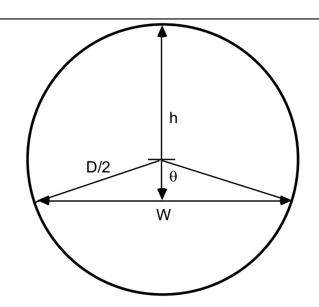
Figure A3.1: Schematic of the Static Load in a Mill
With reference to Figure A3.1:
If the charge width (W) is known, then the fractional filling (J) is given by:
where
$$ \theta $$ = arc sin (W/D) (radians).
If the charge height (h) is known, then the fractional filling is given by:
where
$$ \theta $$ = Arc cos ((2h - D)/D)
APPENDIX 4
D-MODEL PROGRAMME LISTING
| CLS |
|---|
| PRINT "JK-POWER VERSION 1.1.APRIL 1993" |
|
PRINT "THE FOLLOWING IS A PROTOTYPE GRINDING MILL POWER
MODEL DEVELOPED BY" |
|
PRINT
"S.MORRELL OF THE JULIUS KRUTTSCHNITT MINERAL RESEARCH CENTRE(JKMRC)." |
|
PRINT "IT IS A RESEARCH PRODUCT FOR USE BY THE SPONSORS OF THE
JKMRC/AMIRA" |
|
PRINT "MINERAL PROCESSING PROJECT-P9J/K AND IS SUBJECT TO
COPYRIGHT." |
| PRINT "USERS ARE REFERRED TO MORRELL'S PHD THESIS" |
|
PRINT "FOR DETAILS OF THE EQUATIONS AND METHODOLOGY USED
IN THE MODEL." |
|
PRINT
"WHILE REASONABLE CARE HAS BEEN TAKEN IN THE PREPARATION OF THIS " |
|
PRINT
"PROGRAMME NEITHER THE AUTHOR NOR THE JKMRC ACCEPTS ANY RESPONSIBILITY" |
|
PRINT "FOR THE ACCURACY OF THE PREDICTIONS OF GRINDING MILL
POWER THAT IT MAY" |
| PRINT "MAKE" |
PRINT
INPUT "PRESS ENTER KEY TO BEGIN", ST$
IF ST$ = "" THEN 1
1 DIM X(10), y(10), z(21)
10 CLS
cpow = 0: pCAnet = 0: pCTnet = 0: pCnet = 0
REM INPUT DATA
PRINT "MORRELL ' DISCRETE SHELL ' GRINDING MILL POWER MODEL"
PRINT
INPUT "DIAMETER(M)", X(1)
INPUT "BELLY LENGTH(M)", X(2)
INPUT "C/L LENGTH", X(3)
INPUT "RPM", X(4)
INPUT "LIFTER HEIGHT(M)", X(5)
INPUT "TRUNION DIAMETER", X(6)
INPUT "TOTAL FILLING(%)", y(1)
y(1) = y(1) / 100
INPUT "BALL FILLING(%)", y(2)
y(2) = y(2) / 100
INPUT "MEAN MEDIA SIZE(M)", y(3)
MLS = y(3)
INPUT "ORE SG", y(4)
REM input"LIQUID SG",Y(5)
INPUT "DISCHARGE % SOLIDS BY WT", y(6)
INPUT "IS MILL GRATE DISCHARGE(Y/N)?", X$
11 CLS
PRINT "ITERATION UNDERWAY"
REM SET VELOCITY PROFILE PARAMETER
m(1) = .00288: m(2) = .02433
FOR a = 1 TO 2
LGT = X(2)
pnl = 3.47 * (X(2) * X(1) ^ 3 * X(4) / 60) ^ .804
REM mill radius
 z(9) = X(1) / 2
 REM mill rps
 z(4) = X(4) / 60
 REM mill filling
 z(6) = y(1)
 REM vol fraction of pulp
 Cv = y(6) / (y(6) + y(4) * (100 - y(6)))
 REM chg density
 z(7) = (.6 + .4 * Cv) * y(4) + (.6 * y(2) * (7.8 - y(4)) / y(1)) + (.4 * Cv)
 REM pulp density
 z(8) = 100 / (y(6) * (1 - y(4)) / y(4) + 100)
 REM estimate ri
 90 z(11) = X(1) / 2 * (1 - y(1)) ^ .5
 c = 0
 REM adjust ri
 100 z(11) = z(11) + z(11) * c
 REM estimate no. of shells
 m = INT((X(1) / 2 - z(11)) / y(3) - .5)
 REM no. shells influenced by lifter
 li = INT(X(5) / y(3))
 pnet = 0
 FOR n = 1 TO m
 REM z
 z(17) = (1 - z(6)) ^ .4532
 REM fraction crit speed
 z(5) = z(4) * 2 * 3.142 * z(9) ^ .5 / 9.81 ^ .5
 REM actual critical speed
 z(13) = .35 * (3.364 - z(6))
 REM toe angle
 IF n > 1 AND n <= li THEN 102
 z(2) = 2.5307 * (1.279 - z(6)) * (1 - EXP(-(9 * (z(13) - z(5))))) + 1.5708
 IF z(2) < 1.5708 THEN z(2) = 1.5708
REM shoulder angle
 z(1) = 1.5708 - ((.3386 + .1041 * z(5)) + (1.54 - 2.5673 * z(5)) * z(6)) * (z(2) - 1.5708)
 IF z(1) > 1.5708 THEN z(1) = 1.5708
 REM grate or overflow parameters
 102 IF X$ = "y" OR X$ = "Y" THEN z(3) = z(2) ELSE z(3) = 3.299
 IF z(2) < z(3) THEN z(3) = z(2)
 REM net power
 P = .67 * 3.142 * 9.81 * X(2) * z(4) * (z(9) ^ 3 - (z(9) - y(3)) ^ 3) * (z(7) * (SIN(z(1)) -
  SIN(z(2))) + z(8) * (SIN(z(2)) - SIN(z(3))))
 ke = (X(2) * z(7) * z(4) ^ 3 * 3.142 ^ 3 * (z(9) ^ 4 - (z(9) - y(3)) ^ 4))
 IF z(1) = 1.5708 THEN ke = 0
 pnet = pnet + P + ke
 REM shell volume fraction calculations
 REM hn
 z(14) = z(9) * (SIN(z(1)) - SIN(z(2)))
 IF z(14) > 0 THEN 110
 z(15) = 0
 GOTO 120
 REM thn
 110 z(15) = (2 * z(14) / 9.81) ^ .5
 REM tn
 120 z(16) = (2 * 3.142 - z(2) + z(1)) / (2 * 3.142 * z(4))
 REM volume of material in shell
 z(12) = 3.142 * z(4) * y(3) * X(2) * (2 * z(9) - y(3)) * (z(15) + z(16))
 REM load volume of remaider of mill
 z(18) = (z(6) * 3.142 * z(9) ^ 2 * X(2) - z(12))
 REM radial position of next shell (rn)
 z(9) = X(1) / 2 - (n * y(3))
 z(6) = z(18) / (3.142 * z(9) ^ 2 * X(2))
 IF z(6) >= 0 THEN 190
 y(3) = y(3) * .99
 c = 0
 z(4) = X(4) / 60
 z(6) = y(1)
z(9) = X(1) / 2
GOTO 90
REM effect of lifter height
190 IF n <= li THEN 210
REM rps of next shell
z(4) = z(4) * (1 - (z(17) * m(a) / (1 - z(17) * z(11) / z(9))))
210 NEXT n
IF ABS(z(6)) <= .005 THEN 300
c = -(1 * z(6))
pnet = 0
z(4) = X(4) / 60
z(6) = y(1)
z(9) = X(1) / 2
GOTO 100
300 FLS = y(3)
IF a = 1 THEN pTnet = pnet ELSE pAnet = pnet
IF X(3) = X(2) THEN 900
REM CALCULATION OF CONE POWER
REM CONE ANGLE (TC)
TC = ATN((X(3) - X(2)) / (X(1) - X(6)))
REM CONE LENGTH(LC)
LC = (X(3) - X(2)) / 2
y(3) = MLS
REM MAXIMUM NO SLICES ACROSS CONE (TS)
TS = INT(LC / y(3))
pCnet = 0
REM SET MILL FILLING
ML = y(1)
FOR W = 1 TO TS
y(3) = MLS
REM CONE RADIUS
RC = (X(1) / 2) - (W * y(3) / TAN(TC))
IF RC < z(11) THEN 900
304 z(6) = 0
REM ADJUST MILL FILLING
305 ML = ML - z(6)
z(6) = ML
cpow = o
REM SET CONE RADIUS
z(9) = RC
REM SLICE LENGTH
X(2) = MLS
REM RPS
z(4) = X(4) / 60
REM CALCULATE NO. OF SHELLS
m = INT((z(9) - z(11)) / y(3) - .5)
REM no. shells influenced by lifter
li = INT(X(5) / y(3))
FOR n = 1 TO m - 1
IF z(6) > 0 THEN 306
y(3) = y(3) * .99
GOTO 305
REM z
306 z(17) = (1 - z(6)) ^ (.4532)
REM fraction crit speed
z(5) = z(4) * 2 * 3.142 * z(9) ^ .5 / 9.81 ^ .5
REM actual critical speed
z(13) = .35 * (3.364 - z(6))
IF n > 1 AND n <= li THEN 307
REM toe angle
z(2) = 2.5307 * (1.279 - z(6)) * (1 - EXP(-(9 * (z(13) - z(5))))) + 1.5708
IF z(2) < 1.5708 THEN z(2) = 1.5708
REM shoulder angle
z(1) = 1.5708 - ((.3386 + .1041 * z(5)) + (1.54 - 2.5673 * z(5)) * z(6)) * (z(2) - 1.5708)
IF z(1) > 1.5708 THEN z(1) = 1.5708
REM grate or overflow parameters
307 IF X$ = "y" OR X$ = "Y" THEN z(3) = z(2) ELSE z(3) = 3.299
REM net power
P = 2 * .67 * 3.142 * 9.81 * X(2) * z(4) * (z(9) ^ 3 - (z(9) - y(3)) ^ 3) * (z(7) *
 (SIN(z(1)) - SIN(z(2))) + z(8) * (SIN(z(2)) - SIN(z(3))))
ke = 2 * (X(2) * z(7) * z(4) ^ 3 * 3.142 ^ 3 * (z(9) ^ 4 - (z(9) - y(3)) ^ 4))
IF z(1) = 1.5708 THEN ke = 0
cpow = cpow + P + ke
REM shell volume fraction calculations
REM hn
z(14) = z(9) * (SIN(z(1)) - SIN(z(2)))
IF z(14) > 0 THEN 310
z(15) = 0
GOTO 320
REM thn
310 z(15) = (2 * z(14) / 9.81) ^ .5
REM tn
320 z(16) = (2 * 3.142 - z(2) + z(1)) / (2 * 3.142 * z(4))
REM volume of material in shell
z(12) = 3.142 * z(4) * y(3) * X(2) * (2 * z(9) - y(3)) * (z(15) + z(16))
REM load volume of remaider of mill
z(18) = (z(6) * 3.142 * z(9) ^ 2 * X(2) - z(12))
REM radial position of next shell (rn)
z(9) = RC - (n * y(3))
z(6) = z(18) / (3.142 * z(9) ^ 2 * X(2))
IF z(6) >= 0 THEN 390
y(3) = y(3) * .99
GOTO 305
REM effect of lifter height
390 IF n <= li THEN 410
REM rps of next shell
z(4) = z(4) * (1 - (z(17) * m(a) / (1 - z(17) * z(11) / z(9))))
410 NEXT n
IF z(6) <= .01 THEN 800
GOTO 305
800 pCnet = cpow + pCnet
IF a = 1 THEN pCTnet = pCnet ELSE pCAnet = pCnet
NEXT W
900 X(2) = LGT
NEXT a
REM OUTPUT
CLS
PRINT "DIAMETER(M) ", X(1)
PRINT "BELLY LENGTH(M) ", LGT
PRINT "C/L LENGTH(M) ", X(3)
PRINT "% CRITICAL SPEED ", (200 * 3.142 * (X(1) / 2 / 9.81) ^ .5 * X(4) / 60)
PRINT "LIFTER HEIGHT(M) ", X(5)
PRINT "TRUNION DIAMETER(M) ", X(6)
PRINT "TOTAL FILLING (%) ", y(1) * 100
PRINT "BALL FILLING (%) ", y(2) * 100
PRINT "FITTED MEAN MEDIA SIZE(M)", FLS
PRINT "ORE SG ", y(4)
PRINT "DISCHARGE % SOLIDS BY WT", y(6)
IF X$ = "Y" OR X$ = "y" THEN PRINT "GRATE DISHARGE" ELSE PRINT
"OVERFLOW DISHARGE"
REM PRINT "IS MILL GRATE DISCHARGE(Y/N)?", X$
pT = INT(100 * pTnet) / 100
pCT = INT(100 * pCTnet) / 100
NL = INT(100 * pnl) / 100
pT = INT(100 * pTnet) / 100
pA = INT(100 * pAnet) / 100
pCA = INT(100 * pCAnet) / 100
GP = NL + pT + pCT
PRINT " (kW)", " (%)"
PRINT "NET CYLINDER POWER ="; pT, INT(pT * 1000 / GP + .5) / 10
PRINT "NET CONE POWER ="; pCT, INT(pCT * 1000 / GP + .5) / 10
PRINT "NO LOAD POWER ="; NL, INT(NL * 1000 / GP + .5) / 10
PRINT " GROSS POWER ="; GP, 100
PRINT
PRINT "NET IMPACT POWER ="; pA + pCA, INT((pA + pCA) * 1000 /
GP + .5) / 10
PRINT "NET ATTRITION/ABRASION ="; INT(100 * ((pT + pCT) - (pA +
pCA)) + .5) / 100, INT(((pT + pCT) - (pA + pCA)) * 1000 / GP + .5) / 10
PRINT "NO LOAD POWER ="; NL, INT(NL * 1000 / GP + .5) / 10
PRINT " GROSS POWER ="; GP, 100
PRINT
INPUT "HARD COPY"; PR$
IF PR$ = "Y" OR PR$ = "y" THEN 1000 ELSE 1100
1000 LPRINT "MORRELL ' DISCRETE SHELL ' GRINDING MILL POWER
MODEL v1.1"
LPRINT
LPRINT "DIAMETER(M) ", X(1)
LPRINT "BELLY LENGTH(M) ", LGT
LPRINT "C/L LENGTH(M) ", X(3)
LPRINT "RPM ", X(4)
LPRINT "% CRITICAL SPEED ", (200 * 3.142 * (X(1) / 2 / 9.81) ^ .5 * X(4) /
60)
LPRINT "LIFTER HEIGHT(M) ", X(5)
LPRINT "TRUNION DIAMETER(M) ", X(6)
LPRINT "TOTAL FILLING (%) ", y(1) * 100
LPRINT "BALL FILLING (%) ", y(2) * 100
LPRINT "OBS MEAN LOAD SIZE(M)", MLS
LPRINT "FITTED MEAN LOAD SIZE(M)", FLS
LPRINT "ORE SG ", y(4)
LPRINT "DISCHARGE % SOLIDS BY WT", y(6)
IF X$ = "Y" OR X$ = "y" THEN LPRINT "GRATE DISHARGE" ELSE LPRINT
"OVERFLOW DISHARGE"
LPRINT
LPRINT " (kW)", " (%)"
LPRINT "NET CYLINDER POWER ="; pT, INT(pT * 1000 / GP + .5) / 10
LPRINT "NET CONE POWER ="; pCT, INT(pCT * 1000 / GP + .5) / 10
LPRINT "NO LOAD POWER ="; NL, INT(NL * 1000 / GP + .5) / 10
LPRINT " GROSS POWER ="; GP, 100
LPRINT
LPRINT "NET IMPACT POWER ="; pA + pCA, INT((pA + pCA) * 1000 /
GP + .5) / 10
LPRINT "NET ATTRITION/ABRASION ="; INT(100 * ((pT + pCT) - (pA +
pCA)) + .5) / 100, INT(((pT + pCT) - (pA + pCA)) * 1000 / GP + .5) / 10
LPRINT "NO LOAD POWER ="; NL, INT(NL * 1000 / GP + .5) / 10
LPRINT " GROSS POWER ="; GP, 100
LPRINT
1100 INPUT "DO YOU WISH TO RECALCULATE(Y/N)?", U$
IF U$ = "Y" OR U$ = "y" THEN 10
END
APPENDIX 5
ADDITIONAL LIST OF PAPERS RELATED TO GRINDING MILL POWER DRAW
- Barratt D.J., 1979. Semi-Autogenous Grinding a Comparison with the Conventional Route. Proc. Canadian Inst. of Min. Metall. Annual General Meeting.
- Barratt D.J. and Allan M.J., 1986. Testing for Autogenous and Semi-Autogenous Grinding: a Designer's Point of View. Minerals and Metallurgical Processing . May, pp 65-74.
- Fuerstenau D.W., Abouzeid A.Z.M. and Kapur P.C. 1982. Energy Split and Kinetics of Ball Mill Grinding of Mixture Feeds in Heterogenous Environment. Powder Technology , Elsevier-Sequoia, 72, 105-111.
- Fuerstenau D.W., Venkataraman K.S. and Velamakani B.V. 1985. Effect of Chemical Additives on the Dynamics of Grinding Media in Wet Ball Mill Grinding. Int. Journal Mineral Processing, 15, pp 251-267.
- Goldman M., Barbery G. and Flament F., 1991. Modelling Load and Product Distribution in Autogenous and Semi-Autogenous Mills: Pilot Plant Tests, CIM Bulletin , Vol 84, No 946, pp 80-86.
- Guerrero P.K. and Arbiter N., 1960. Tumbling Mill Power at Cataracting Speeds. Trans. SME/AIME , vol. 217, pp 73-75.
- Harris C.C. and Arbiter N., 1982. Grinding Mill Scale-up Problems, Mining Engineering, Vol 34, No 1, pp 43-46.
- Harris C.C. and Arbiter N., 1985. Grinding Mill Operation and Scale-up: Theory and Equations. Mineral Processing and Technology Review , Vol 1, pp 249- 263.
- Herbst J.A. and Rajamani K., 1982. Developing a Simulator for Ball Mill Scale-up: a Case Study. Design and Installation of Comminution Circuits , Mular A.L. and Jergensen G.V. (eds), AIME, New York, Ch 20, pp 325-342.
- Jenness R.C., 1972. Rotary Grinding Mill and Drive Motor Torque Relationships. Proc. Cement Industry Technical Conference , Detroit, Michigan. (Also Allis Chalmers Publication 07P4734).
- Lukasiewicz S.A., Swisterski W. and Romaniszyn G., 1990. Supercritical Revolutions of Tumbling Mills. Minerals and Metallurgical Processing, pp 100-106.
- Mishra B.K. and Rajamani Raj K., 1992. The Discrete Element Method for the Simulation of Ball Mills. Appl. Math. Modelling , Butterworth-Heinemann, Vol 16, November, pp 598-604.
- Mokken A.H., 1978. Progress in run-of-mine (autogenous) milling as originally introduced and subsequently developed in the gold mines of the Union Corporation Group. Proc. 11th Commonwealth Mineral and Metallurgical Congress, M.J. Jones (ed), Inst. of Min. Metall., London, paper 49.
- Moller T.K. and Brough R., 1989. Optimizing the Performance of a Rubber-lined Mill. Mining Engineering , August, pp 849-853.
- Morrell S., Napier-Munn T.J. and Andersen J., 1992. The Prediction of Power Draw in Comminution Machines. Comminution - Theory and Practice, K. Kawatra (ed), SME. Ch 17, pp 235-247.
- Parks J.L. and Kjos D.M., 1990. Liner Designs, Materials and Operating Practices for Large Primary Mills. CIM Bulletin, Vol 83, No 943, pp 84-89.
- Powell M.S., 1990. Improving the Design of the Liners of Rotary Mills. Proc. International Deep Mining Conference. Innovations in Metallurgical Plant. Johannesburg, SAIMM, pp 57-70.
- Rowland C.A., 1975. The Tools of Power: How to evaluate grinding mill performance using the Bond Work Index to measure grinding Efficiency. Proc. AIME Annual Meeting , Tuscon, Arizona.
- Rowland C.A., 1981. Pilot Plant Data for the Design of Primary Autogenous and Semi-Autogenous Mills. Proc. Canadian Inst. Min. Metall. 83rd Annual General Meeting, Calgary, preprint 99.
- Rowland C.A. and Kjos D.M., 1978. Plant Design Considerations for Rod and Ball Mill Grinding Circuits. Minerals Processing Plant Design . Mular and Bhappu (eds), AIME, Ch 12, pp 239-278.
- Sandvik K.L., 1991. Design Criteria for large Mills partly based upon the experiences with the Sydvaranger 6.5 x 9.65 m ball mill. Preprints XVII IMPC , Dresden, Vol 1, pp 165-176.
- Steane R.A. and Hinkfuss D.A., 1973. The Selection and Performance of Large Diameter Ball Mills at Bougainville Copper Limited. Proc. 11th Commonwealth Mineral and Metallurgical Congress , M.J. Jones (ed), Inst. of Min. Metall., London, pp 577-584.