USING MODELLING AND SIMULATION FOR THE DESIGN OF FULL SCALE BALL MILL CIRCUITS

S Morrell and Y T Man

ABSTRACT

Computer simulation of ball mill cicuits has been found to be very valuable for optimisation where existing plant data can be used to calibrate the mathematical models used. However, as by definition no existing plant is available for calibration in greenfield scenarios, the use of simulation in ball mill circuit design has been limited. Running a pilot ball mill circuit can overcome this problem but this requires a reasonably large sample and therefore can be costly. In addition a valid scale-up procedure is required. To overcome these limitations in using modelling and simulation for designing ball mill circuits, a programme of research was initiated at the JKMRC in which it was proposed to use laboratory ball mill test results to calibrate a suitable ball mill mathematical model for use in predicting full scale plant performance. To validate the technique, laboratory tests were conducted on a range of ore samples from existing plants, whose ball mill circuits were surveyed. The model, which was derived from the laboratory test results was then used to predict the full scale plants' performance. This paper describes the technique used and gives initial results from the comparison between the model predictions and the results obtained from the full scale plants.

INTRODUCTION

Despite the widespread use of simulation for optimising ball mill circuits its use in greenfield design remains limited. This is in contrast to autogenous (ag) and semiautogenous (sag) mill circuits where simulation techniques are now used as standard in most design projects. Undoubtedly the limited inroads that simulation has made in ball mill circuit design is due to the historic success of Bond's method [1] in crusher–ball mill and rod mill–ball mill circuits. Unfortunately Bond's method is limited to providing the required mill power draw for a given duty. In doing so it relies on certain assumptions, including the shape of feed and product size distributions, which should be parallel on a log–log scale, and the efficiency of the classifier, which is taken to be perfect. However, the popularity of circuits comprising ag and sag mills followed by ball mills has presented Bond's method with some problems. This is due to the fact that typical ag/sag mill product size distributions do not usually follow those of rod mills and crushers which Bond used when formulating his equations. Figure 1 shows a size distribution of the product from a sag mill ahead of a ball mill. Superimposed is a distribution with a similar P80 but from a crushing plant feeding a ball mill. Also plotted are the cyclone overflows from each circuit.

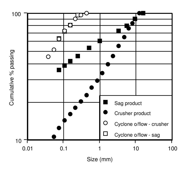
Differences are apparent in the finer size fractions which show that the sag mill product contains a considerable amount of final product, in contrast to the crusher product. The cyclone overflows are almost identical for the two circuits and are parallel on a log–log scale to the crusher product – as per the requirement for application of the Bond equation. This is not the case for the sag mill data. The implication of these differences is that the Bond method may not be valid for sizing ball mill circuits which follow an ag/sag mill circuit. This limitation is recognised by some designers who modify the ag/sag mill product size prior to applying Bond's formula for sizing the ball mill. Whereas such modifications may improve the accuracy of the Bond method for sizing ball mills it remains a technique which is not directly compatible with, and therefore lacks the versatility of, modern simulation.

The recognised strength of simulation lies in its ability to assess the performance of an entire comminution circuit and to determine the interaction between the various units in the circuit. This enables the designer to change the configuration of the proposed circuit as well as the size of the equipment and the way they are operated to ensure that the design is an efficient one. In addition the simulation provides details of all the flows around the circuit including full size distributions and water contents. Providing the models are lifelike they should not suffer from the limitations of Bond's techniques and hence should be applicable regardless of the feed size distribution and operating conditions of the units in the circuit. The problem facing the designer, particularly at the pre-feasibility stage, is what model should be chosen to ensure a realistic prediction of the behaviour of a full scale ball mill.

The most commonly used ball mill model structure is that based on the population balance approach [2]. This very versatile model has at least one major drawback in that its parameters cannot be determined a priori but must be fitted to data from an existing circuit. Clearly in the greenfield plant design scenario no such plant exists. Piloting is obviously one option but this requires a relatively large ore sample which, in the early stages of development of the deposit, may not be available. In addition a scale-up procedure to allow the use of the pilot data must also be established. Laboratory scale milling testwork solves the problem of sample quantity, though as with piloting, scale-up is still an issue. Some researchers have suggested modelling/scale-up procedures [3-5]. Unfortunately data on their widespread validity are either limited or non-existent, or it has been concluded that direct scale-up from small scale tests is not possible [6]. Partly because of this the Minerals Processing Industry has not embraced this technology to any great extent for design of ball milling circuits.

To overcome the reluctance of industry to use modelling and simulation in ball mill circuit design and hence realise the full potential of this technique, a research project was initiated at the JKMRC. Its objective was to establish a simple laboratory based methodology which would generate the required model parameters which could then be used with confidence to scale-up to any size of mill under normal operating conditions. This paper presents the initial results from this project.

MODELLING

Given the requirement for developing a model which could be used for design in greenfield scenarios it was initially decided to use a relatively simple structure. To this end Whiten's so called perfect mixing model was used [7]. In its complete form it comprises two equations as follows:

$$ \frac{ds_{i}}{dt} = f_{i} - p_{i} + \sum_{j=1}^{i} b_{ij} r_{j} s_{j} - r_{i} s_{i} $$ (1)

where:

\( f_i \) = feed rate of size fraction i (t/hr)

\( p_i \) = product flow of size fraction i (t/hr)

\( b_{ij} \) = the mass fraction of particle of size that appear at size i after breakage

\( r_j \) = breakage rate of particle size j (hr^-1)

\( s_j \) = amount of size j particles inside the mill (tonnes)

t = grinding time (hr)

The value of the mill contents is very difficult to determine experimentally. Therefore the mill contents component, \( s_i \) , is eliminated by combining equations 1 and 2. Thus:

$$ \frac{ds_{i}}{dt} = f_{i} - p_{i} + \sum_{i=1}^{i} b_{ij} \frac{r_{j}}{d_{i}} p_{j} - \frac{r_{i}}{d_{i}} p_{i} $$ (3)

At steady state \( \frac{ds_i}{dt} \) is zero, therefore:

$$ 0 = f_{i} - p_{i} + \sum_{j=1}^{i} b_{ij} \frac{r_{j}}{d_{j}} p_{j} - \frac{r_{i}}{d_{i}} p_{i} $$ $$ (4) $$

Hence, given a feed size distribution the product size can be predicted using Equation 4 providing the \( b_{ij} \) and the \( r_i/d_i \) are known.

Residence Time

Implicit in this model is the assumption that the mill is a single perfectly mixed reactor, though classification effects can be accommodated by variation in the discharge rate parameter (d_i). The assumption of a single perfectly mixed reactor can be criticised due to the results from liquid tracer tests which show that a series of unequal mixers more closely fits experimental residence time data. For example Weller et al [5] found that the number of mixers in series which fitted their residence time data varied in the range 3 – 5, with the largest mixer accounting for 0.2 – 0.95 of the total residence time. Further ball mill data presented by Weller [8] shared the same characteristics in that their residence time distributions could be fitted well by a series of perfect mixers. However it was noteworthy that this fitting was done with "no constraints on their (mixers) relative sizes". The consequential lack of a physical relationship between the mill design and the mixer configuration is a serious drawback of this approach, particularly in greenfield design situations where the designer must choose a suitable configuration. In such cases, if it is not possible to predict what the required mixer-in-series configuration should be for a given mill, the assumption of a single perfectly mixed reactor is an obvious choice. Initially, therefore, it was decided to use this assumption.

Breakage Rate and Appearance Functions

The bij are the breakage distribution or appearance function values which describe the size distribution of the progeny following breakage. In the case where i=j, bij is defined as the fraction of the original particle remaining in its size class after breakage. Hence (1-bkk) is the fraction broken out of size class k. In most ball mill models the breakage distribution function is assumed, for mathematical convenience, to be both normalisable and invariant with respect to mill design and operating conditions. However, from studies of single particle breakage it has been found [9] that for a given size class the bij are dependent upon specific energy input. It is logical to assume that as mill diameter increases the energy available for breakage increases and hence the breakage distribution function will not be constant but will change with mill conditions. For a given ball size this breakage energy will be related to the density of the balls and the height from which they drop, which in turn will be related to mill diameter.

Hence:

where:

Dm = mill diameter

ρb = grinding media density

From Equation 4 the relevant expression for describing breakage out of a given size class (k) is:

Breakage out of size class $$ k = \frac{r_k}{d_k} (1 - b_{kk}) $$ (6)

The breakage rate (rk) can be defined as the number of breakage collisions per particle per unit time ie. it is the expected frequency that a given particle will be hit by a ball [10]. Its dependence is therefore on the rate at which the mill rotates, the volume of balls in the mill, and the slurry hold-up.

Hence:

$$ r_k \propto \frac{V_B N}{V_{\text{pulp}}} $$ (7)

where:

L = mill length

N = rotational rate of the mill

V ^B = volume of balls

JB = fractional mill filling with balls

Vpulp = slurry hold-up

The discharge rate (dk) is given by Equation 2. If there is no segregation in the mill, then solid particles will behave like water and dk will be invariant with respect to size, in which case dk is constant and is given by:

Combining equations 6 – 9 gives the dependence of the breakage term as follows:

$$ (1 - b_{kk}) \frac{r_k}{d_k} \propto \frac{D_m \rho_b N J_B D_m^2 L V_{pulp}}{Q_{pulp} V_{pulp}} $$ (10)

The numerator in proportionality 11 is a simple expression for power draw, whilst the denominator is the volumetric flowrate out of the mill. The units of the expression are therefore proportional to kWh/m3. This result is consistent with the experimental findings of Herbst and Fuerstenau [11] in their laboratory based work which concluded that specific energy (kWh/t) was proportional to the breakage function.

As the mill diameter or ball size increases the energy delivered by a ball as it is lifted and dropped by the rotation of the mill will also increase. Therefore the breakage distribution function can be expected to change. However, mathematically it is convenient to keep the breakage distribution function constant and incorporate the effects of scale in the variation of the rk/d ^k parameter. Hence the scaling becomes:

where:

P = net mill power, ie. power at the shell.

Power Draw

The dependence of the scaling on power necessitates accurate prediction of mill power. The JKMRC has developed a power model [12] which has been proven using a wide range of data. The model uses a simplified description of the grinding charge motion and incorporates the effects of the slurry pool which forms in all overflow mills and in some grate discharge mills at high flowrates [13-14].

The model incorporates equations which describe the position of the shoulder and toe of the charge and how they change as speed and volumetric loading vary. The model uses these calculations in an energy balance which, together with the rotational rate, provide the power drawn by the mill at the shell. A separate equation is then used to estimate motor, gearbox and bearing losses which are added to the power to give gross power.

Ball Size Effects

Although the power delivered to the mill shell can be predicted accurately by the power model it is the power delivered to the slurry charge which is important in determining how much grinding takes place. Power at the mill shell is transferred to the slurry charge via the grinding balls, the size distribution of which affects how this occurs. Therefore it is necessary in proportionality 12 to incorporate the effect of ball size.

This is done by considering that breakage in ball mills occurs due to direct impact of balls on rock particles as well as that caused when rock particles are nipped and crushed between balls as they roll/slide over one another (attrition). In the case of impact breakage the kinetic energy of a grinding ball (and hence its mass) will be directly related to the amount of breakage it will cause.

Thus:

amount broken $$ \propto $$ ball mass (13) \( \propto D_b^3 \)

where:

D ^b = ball diameter

In the case of attrition grinding the amount broken will not be dependent upon individual ball masses but upon the pressure exerted by the ball bed [15]. In both cases the amount of ball surface will also directly affect the amount of breakage as it will determine the amount of grinding surface between which particles can be reduced in size. Thus for a fixed ball volume:

Total ball surface area $$ \propto D_b^{-1} $$ (14)

For impact breakage, therefore, proportionalities (13) and (14) combine to give:

Impact breakage $$ \propto D_b^2 $$ (15)

whilst for attrition:

Attrition breakage $$ \propto D_b^{-1} $$ (16)

For attrition breakage to occur a particle must be small enough in relation to the grinding media to be nipped, hence proportionality (16) can only be applied for particles below a size which is related to the grinding media size.

The classical breakage rate distribution that is normally obtained from mill feed and product data (Figure 2) can be interpreted in the light of the breakage modes of impact and attrition. Given that attrition can only affect particles smaller than a certain size then the peak in the breakage rate distribution will be associated with ball size. It is therefore hypothesised that for particles below the size associated with this peak attrition breakage will predominate, whilst above this size impact breakage will. The size at which this peak occurs \( (x_m) \) has been suggested by Austin et al. [4] to be related to ball size in the following way:

or

From a range of industrial mills in the JKMRC data base it has been found that Equation 18 is valid and that K is approximately equal to 0.00044, where the units of \( x_m \) and \( D_b \) are expressed in mm.

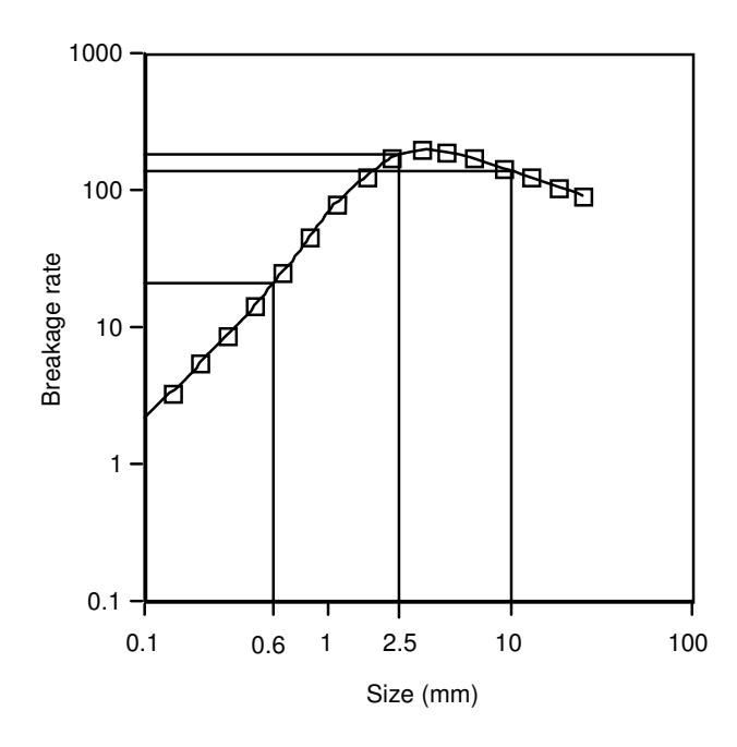
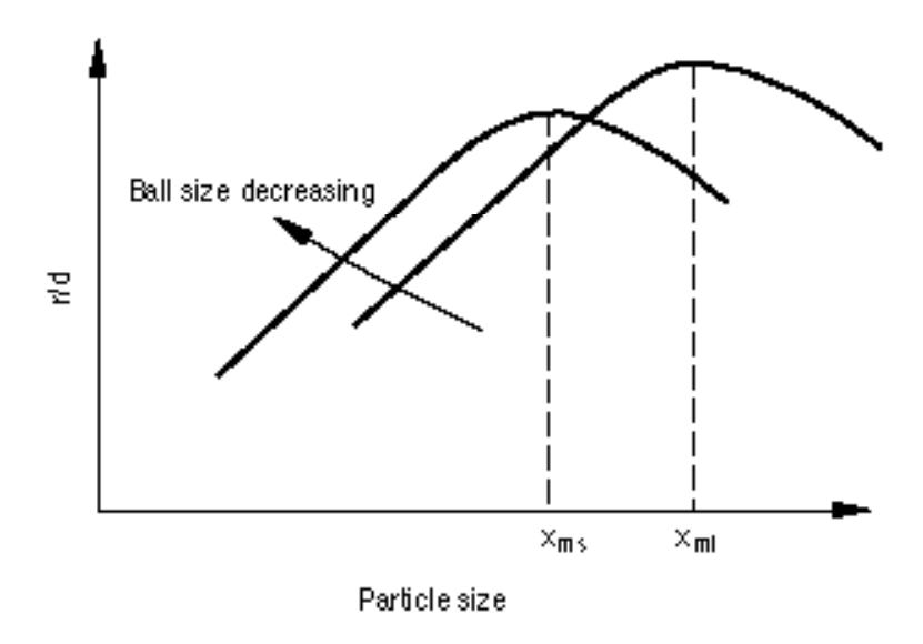
It is convenient to describe the breakage rate distribution using splines [16]. Three or four spline knots are normally required, each knot having a breakage rate value and an associated particle size. Hence in Figure 2 the breakage rate distribution is described by breakage rate values at particle sizes of 0.6, 2.5 and 10mm. Using the impact and attrition dependencies described earlier, an algorithm was devised in which the spline knot values were varied according to the ball size. In this way the effect of changing ball size on the breakage rate distribution was accommodated. The algorithm relies on identifying the xm value associated with the original ball size and new ball size, the effects of which require to be predicted. Hence, with reference to Figure 3, if an increase in ball size is required to be predicted then for all knot sizes less than xms the breakage rates are multiplied by the attrition breakage factor:

Dbs Dbl

where:

Dbs = the original (smaller) ball size

Dbl = the new (larger) ball size, and

xms = the particle size associated with the peak breakage rate of the original ball size.

For knot sizes greater than xml the breakage rates are multiplied by the impact breakage factor:

where:

\( x_{ml} \) = the particle size associated with the peak breakage rate of the new ball size.

In this way a new set of breakage rates for each spline knot are predicted. Using splines a smooth curve is then drawn through each new point, thus generating a new breakage rate distribution.

SCALE-UP PROCEDURE

The power, flowrate and ball size dependencies described in the previous section can be summarised as follows:

where:

$$ P = net power draw $$ \( Q = volumetric flowrate \) \( \beta_i = \frac{r_i}{d_i} \)

\( f(D_b) \) = complex function of \( D_b \)

whilst from Equation 4:

$$ p_{i} = f_{i} + \sum_{j=1}^{i} b_{ij} \beta_{j} p_{j} - \beta_{i} p_{i} $$ (20)

If, in a test mill, the \( \beta_i \) , P, Q, \( D_b \) and \( b_{ij} \) can be measured/calculated and P, Q and \( D_b \) estimated for the full scale mill, then \( \beta_i \) for the full scale mill can be determined from Equation 21. Equation 20 can subsequently be used to predict the product of the full scale mill.

$$ \frac{\beta_{i \text{ Full scale}}}{\beta_{i \text{ Bond}}} = \frac{P_{\text{Full scale}} Q_{\text{Full scale}}^{-1} f(D_b)_{\text{Full scale}}}{P_{\text{Bond}} Q_{\text{Bond}}^{-1} f(D_b)_{\text{Bond}}} $$ (21)

In this work the Bond mill was the test mill. Despite the limitations of Bond's technique, it remains a very valuable tool for the ball mill circuit designer, particularly as a means for comparing the grindability of ores. Hence the huge data bases of Bond ball work indices that have been built up by various organisations around the world will most likely ensure that the Bond laboratory test remains a standard for a long time to come. With this in mind it was decided to use Bond's laboratory ball work-index test to generate data for determining relevant model parameters. This approach had the advantage that it required only small quantities of ore which could be used simultaneously to generate a Bond work index as well as the required model parameters. It is emphasised that the Bond work index is not used in the scale-up procedure. The scale-up procedure requires sizing data from the Bond ball mill test, the breakage function (appearance function) of the material to be ground, the volumetric flow of slurry to the full scale mill, and the dimensions and operating conditions of the full scale mill.

ASSESSMENT OF THE SCALE-UP PROCEDURE

Samples of fresh feed were taken from each of the feed streams to 6 different full scale ball mills. In each case the mills were fed with sag mill discharge. At the same time detailed surveys of all 6 mill circuits were conducted. Details are given in Table 1.

Table 1: Summary of the mill survey conditions and Bond test results

	Scuddles	MIM Cu	OK Tedi
		Concentrator	Mill 1A	Mill 1B	Mill 2A	Mill
			2B
Diameter (m)	3.81	5.03	4.77	4.87	4.87	5.33
Length (m)	6.70	6.10	8.84	8.84	8.84	8.54
Fract. cr. speed	0.78	0.70	0.72	0.75	0.75	0.72
Load fraction	0.37	0.41	0.30	0.30	0.30	0.30
Ball size (mm)	80/50	55	50	50	50	50
Feedrate (t/hr)	120	526	910	1592	1028	1571
Solids s.g.	4.0	2.9	2.6	2.6	2.6	2.6
Mill Power (kW)	1240	2540	3600	3250	3200	3740
Bond WI (kWh/tonne)	11.7	17.6	10.6	10.6	10.8	10.8

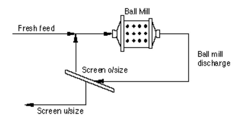
Using the feed samples Bond laboratory tests were conducted. For each sample the size distribution of the last cycle's closing screen undersize and oversize, together with the sizing of the fresh feed and the net grams of final product generated per revolution, were used to create a mass and size balance around this "circuit". Although the Bond test is not fully continuous, its structure ensures that it comes to approximate equilibrium. At this time the test approximates the steady state performance of a closed-circuit continuous mill with a recycle load of 250%. The process flow sheet of a Bond test, when envisaged as a continuous operation is represented by Figure 4. Table 2 gives details of the Bond laboratory ball mill.

Table 2: Bond ball mill details

Diameter (m)	0.305
Length (m)	0.305
Speed (rpm)	70
Speed (fr. crit)	0.91
Ball load (%)	19.3
Ball top size (mm)	36.4

Feed samples were also subjected to a series of single particle breakage tests. These were conducted at a range of specific energies using a drop-weight device [17]. From these results breakage distribution functions were determined using an arbitrary specific energy input of 1 kWh/t. Using this and the mass balance of the Bond test "circuit" Equation 20 was used to back calculate the βi .

In Equation 21 the mean volumetric flow out of the Bond mill is required. Since the volume of ore ground in the Bond test is 700ml, the mean volumetric flow through the Bond mill is:

$$ Q_{Bond} = \frac{0.007}{\text{duration of the last cycle (hour)}} \text{ m}^3/\text{hr} $$ (22)

From each of the Bond tests the duration of the last cycle was used to determine QBond.

The net power drawn by the Bond mill also needs to be established. As the Bond mill has no lifters, the JKMRC power model [12] cannot be used in its normal form. This is because this model was derived from experiments using mills with lifters. However, earlier studies by Morrell [18] provided charge motion data for smooth mills such as the Bond mill. These data were therefore used to construct a power model for smooth mills. This model was then used to predict the net power draw of the Bond mill. The resultant prediction of the new power draw of the Bond mill was 86.65W, which is comparable to Levin's [19] value of 86.4W.

From the full scale mill dimensions and operating conditions, the net mill power draw was predicted using the JKMRC power model [12]. As the volumetric flowrate and ball top size of the full scale mills were measured, the βi for the full scale mills were determined from Equation 21. Equation 20 was then used to predict the product size distribution of the full scale mill for a given feed size distribution.

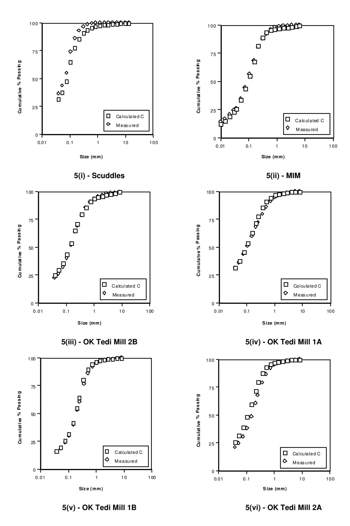
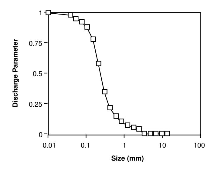
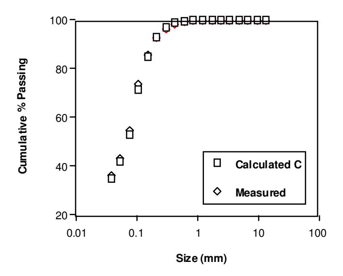
The measured product size distributions from the surveys and the predicted ones using the scale-up technique are shown in Figure 5. It can be seen that agreement is reasonable, with the OK Tedi mill 2A and Scuddles being the least satisfactory. In the case of the OK Tedi data it is pointed out that the mills treat very large flowrates and consequently plant sampling was particularly difficult. In addition it was not possible to measure the ball load and instead the mill operator's estimate had to be used. The measured data are therefore likely to contain sampling errors higher than normally expected. In the case of the Scuddles mill it is of note that it is a relatively low throughput mill and a high s.g. ore. Despite a reasonably coarse feed, its product contained little or no material larger than 0.5 mm. It is possible that due to the resultant low superficial velocity of slurry through the mill and high solids s.g., coarser material was prevented from exiting the mill and accumulated in the holdup. In the model, classification within the mill is assumed not to occur. However if the classification curve shown in Figure 6 is incorporated within the model the prediction given in Figure 7 is obtained. This shows excellent agreement with the measured results. More data are currently being collected to confirm whether classification of this nature occurs in mills with relatively low throughputs and/or coarse feeds, and if so what is the most appropriate way to model it.

To illustrate how the procedure is applied a worked example is given in the Appendix. Obviously in a greenfield design situation the volumetric flowrate to the mill would be obtained from the specified water addition rate, new feedrate plus the recycle from the classifier which would be predicted by the simulation. Ball size would be specified by the designer as would mill dimension, speed etc. These would be adjusted by the designer, together with the classifier performance, until the required grind size was reached.

CONCLUSIONS

A method for predicting full scale ball mill performance has been developed which is based on laboratory tests only. It combines the Bond Work Index test with population balance and mill power models. The method incorporates the effects of all major variables such as dimensions, mill speed, ball load and ball size and flowrate. Comparison of the predicted and measured discharge size distributions from a number of large diameter mills has shown that the method shows promise.

Further work is needed to validate the method, particularly in the treatment of classification within the mill. Additionally, the method needs to be tested with mills which receive a larger range of feed sizes, such as those treating crushing plant product and regrind mills. This work is currently underway.

ACKNOWLEDGMENTS

The finacial support of the sponsors of the AMIRA-JKMRC projects P9K and P9L, in particular OK-Tedi Minig Ltd., MIM Ltd. and Murchinson Zinc Ltd., is gratefully acknowledged. The authors also wish to thank Dr W.J. Whiten for his advice on the Whiten's perfect mixing model and assistance in computer programming.

REFERENCES

• 1. Bond, F.C., Cushing and Grinding Calculations, Allis-Chalmers Publication, No. 07R9235B (1961).
• 2. Epstein, B., The Material Description of Certain Breakage Mechanisms leading to the Logorithmic-Normal Distribution, J. Franklin Inst. (1947).
• 3. Herbst, J.A. and Fuerstenau D.W., Scale-Up procedure for Continuous Grinding Mill Design Using Population Balance Models, International Journal of Mineral Processing, Vol. 7, pp 1-31, (1980).
• 4. Austin, L.G., Luckie, P.T., and Klimpel, R.R., The Process Engineering of Size Reduction: Ball Milling, S.M.E./AIME, New York, 561 pp (1984).
• 5. Weller K.R., Sterns U.J., Artone E. and Bruckard W.J., Multicomponent Models of Grinding and Classification for Scale-Up from Continuous Small or Pilot Scale Circuit, International Journal of Mineral Processing, Vol. 22, pp 119-147 (1988).
• 6. Austin, L.G. and Weller K.R., Simulation and Scale-Up of Wet Ball Milling, CIM XIV International Mineral Processing Congress, October 17-21, TORONTO, pp I-8.1 to I-8.2 (1982).
• 7. Whiten, W.J., A Matrix Theory of Comminution Machines, Chemical Engineering Science, Vol. 29, pp 31-34 (1974).

• 8. Weller, K.R., Hold-Up and Residence Time Characteristics of Full Scale Grinding Circuits, IFAC Mining, Mineral and Metal Processing, Montreal, pp 303-309, (1980).
• 9. Narayanan, S.S. and Whiten W.J., Breakage Characteristics for Ores for Ball Mill Modelling, Proceeding of the Australasian Institute of Mining and Metallurgy, No. 286, pp 31-39, June (1983).
• 10. Morrell, S., Simulations of Bauxite Grinding in a Semi-autogenous Mill and DSM Circuit, MEng Thesis, The University of Queensland (1989).
• 11. Herbst, J.A. and Fuerstenau D.W., Mathematical Simulation of Dry Ball Milling using Specific Power Information, Transaction. SME-AIME, Vol. 254, pp 343-348 (1973).
• 12. Morrell, S., Power Draw of Wet Tumbling and Its Relationship to Charge Dynamics - Part 1: A Continuum Approach to Mathematical Modelling of MillPower Draw, Transaction of the Institution of Mining and Metallurgy; Section C, Vol. 105, pp C43-C53 (1996).
• 13. Moys, M.H., Van Nierop, M.A. and Smit, J., Progress in Measuring and Modelling Load Behaviour in Pilot and Industrial Mills, Minerals Engineering, Vol. 9, No. 12, pp 1201-1214 (1996).
• 14. Morrell, S. and Kojovic, T., The Influence of Slurry Transport on the Power Draw of Autogenous and Semi-autogenous Mills, Proc. SAG '96, Vol. 1, pp 373- 389 (1996).
• 15. Kelly, E.G. and Spottiswood D.J., The Breakage Function; What Is It Really?, Minerals Engineering, Vol. 3, No. 5, pp 405-414 (1990).
• 16. Ahlberg, J.H., Nilson E.N. and Walsh J.L., The Theory of Splines and Their Applications, Mathematics in Science and Engineering, Vol. 38, Academic Press, New York and London (1967).
• 17. Napier-Munn, T.J., Morrell S., Morrison R.D. and Kojovic T., Mineral Comminution Circuits: their Operation and Optimisation, JKMRC Monograph Series in Mining And Mineral Processing 2 (1996).
• 18. Morrell, S., Prediction of Grinding Mill Power, Transaction of the. Insitution of Mining and Metallurgy, Section C, Vol. 101, pp C25-32 (1992).

19. Levin, J., Observation on the Bond Standard Grindability Test, and a Proposal for a Standard Grindability Test for Fine Materials, Journal of South African Institute of Mining and Metallurgy, Vol. 89, No. 1, pp 13-21 (1989).

APPENDIX

To illustrate the use of the scale-up method a worked example is given. The equation numbers given in the calculation steps refer to the equations of the main text.

Input Data

The scale-up method requires the following data:

Bond test data – Mill feed size distribution (ie. new feed plus final recycled screen oversize - see Table A1)

– Final mill discharge size distribution (see Table A1)

– Duration of last cycle - 0.096 hours

Full scale mill data – Mill feed size distribution (see Table A1)

– Feed rate - 526 t/hr

– Discharge slurry % solids by volume - 50%

– Mill diameter - 4.85m – Mill length - 5.92m

– Mill speed - 73% of critical

– Ball size - 55mm

– Ball load - 41% of mill volume

Ore data – s.g. - 2.85

– Appearance function (see Table A1)

Calculation Steps

1: Calculate the breakage rate parameter for the Bond mill, βi Bond Input data: Appearance function, final mill feed and mill discharge from Bond test as given in Table A1 in columns 2, 3, and 4 respectively.

From Equation 4 the βi Bond values are calculated. The resultant distribution is shown in Table A1, column 5. 2: Adjust \( \beta_i \) for difference in top ball size between the Bond laboratory mill and full scale mill

Input data: \( \beta_{i \text{ Bond}} \) , the top ball size for the Bond laboratory mill \( D_{bs} \) = 36.4mm; top ball size for the full scale mill \( D_{bl} \) = 55mm.

From Equation 18: \( x_{ms} = 0.58 \) mm, \( x_{ml} = 1.33 \) mm

For particle sizes greater than or equal to \( x_{ml} \) the \( \beta_{i \; Bond} \) values are multiplied by the impact breakage factor \( \left(\frac{D_{\; bl}}{D_{\; bs}}\right)^2 \) . For particle sizes smaller than or equal to \( x_{ms} \) the \( \beta_{i \, Bond} \) values are divided by the attrition factor \( \left(\frac{D_{\, bl}}{D_{\, bs}}\right) \)

For \( \beta_{i\ Bond} \) values between \( x_{ml} \) and \( x_{ms} \) , a spline function is used to give a continuous and smooth curve. The resultant breakage rate parameter is given in Table A1, column 6.

3: Calculate the net power draw of the full scale mill, \( P_{Full \ scale} \) Input data: design and operating data of the full scale mill. Using the Morrell power model (1996) the net power draw of the mill is calculated to be:

4: Calculate Q_Bond

Input data: Duration of last cycle of the Bond test. From Equation 22 \( Q_{bond} = 0.007/0.096 \) = \( 0.007259m^3/hr \)

5: Calculate \( \beta_{i \text{ full scale}} \)

Input data: \( P_{Bond} = 0.08665 \) kW using Morrell power model for smooth mills (1992), \( P_{Full\ scale} = 2456 \) kW, volumetric flowrate of the Bond mill \( Q_{Bond} = 0.007259 \) m³/h, volumetric flowrate of the full scale mill \( Q_{Full\ scale} = 369 \) m³/h.

Multiply ball size-adjusted \( \beta_{i\;Bond}\; \) values by the scaling ratio

The resultant breakage rate parameter for the full scale mill, \( \beta_{i \text{ Full scale}} \) is given in Table A1, column 8. 6: Calculate the mill discharge size distribution of the full scale mill Input data: The feed size distribution of the full scale mill (column 9), the \( \beta \) i Full scale values (column 8) and the appearance function (column 2).

Using Equation 4 the mill discharge size distribution for the full scale mill can now be calculated and is given in column 10.