THE MORRELL METHOD TO DETERMINE THE EFFICIENCY OF INDUSTRIAL GRINDING CIRCUITS

REVISED 2021 FIRST PUBLISHED 2016 INDUSTRIAL COMMINUTION EFFICIENCY

Global Mining Guidelines Group (GMG)

CREDITS

While many organizations and individuals were involved in the preparation of these guidelines at various stages, please note that the guidelines do not necessarily represent the views of the organizations involved.

Project Group

The Morrell Method to Determine the Efficiency of Industrial Grinding Circuits (Revision 2)

Subcommittee

Industrial Comminution Efficiency

Working Group

Mineral Processing

Project Leader

Mike Daniel, CMD Consulting

Revision Committee

Guillaume Chiasson, SGS Steve Morrell, SMC Testing

FOREWORD

The Morrell method is well known and widely applied in the design of comminution circuits. This guideline provides readers with a practical, condensed version of the Morrell method. The guideline reviews the data required for analysis including hardness characterization data generated from the SMC Test® and the Bond Ball Mill Test Work Index, and the Morrell equations and their applications. This guideline is intended for those looking for a detailed breakdown of the Morrell method and equations.

The Morrell method can be applied for the design and optimization of comminution circuits. The method essentially consists of two parts:

• Part 1: Power draw modelling of equipment such as ball mills and autogenous grinding (AG) and semiautogenous grinding (SAG) mills.
• Part 2: Using ore properties to assess the circuit specific energy. This can also include assessment of the specific energy requirements for crushing, high pressure grinding roll (HPGR), and tumbling mill processes.

In context to this guideline, the Morrell method is used to predict specific energy of comminution circuits that include combinations of equipment including:

• Autogenous grinding (AG) and semi-autogenous grinding (SAG) in autogenous ball milling crushing (ABC), semi-autogenous ball milling (SAB) and semi-autogenous ball milling crushing (SABC) circuits
• Crushers and ball mill circuits
• Crushers, HPGRs, and ball mill circuits (2C/HPGR/BM)

Although the Morrell method is mostly used in comminution circuit design in greenfield projects, this document provides guidance to use the method to assess the energy utilization efficiency of existing circuits.

Overall, this methodology is the comparison of measured and modeled values to determine the efficiency.

ABBREVIATIONS

AG Autogenous Grinding

F80 80% passing size of the circuit feed (μm)

Gpb Grams (new minus closing screen aperture) per mill revolution (laboratory ball mill)

HPGR High Pressure Grinding Roll

Mi Generic term for hardness parameters Mia, Mib, Mic, and Mih

Mia Coarse ore (> 750 μm) work index in tumbling mill circuit(s) (kWh/t) Mib Fine material (< 750 μm) work index in tumbling mill circuit(s) (kWh/t)

Mic Ore work index in crusher circuits (kWh/t) Mih Ore work index in HPGR circuits (kWh/t)

P100 100% passing size or closing screen aperture (μm)

P80 80% passing size of the circuit product (μm)

S General term for coarse ore hardness parameter

Sc Coarse ore hardness parameter for conventional crushing Sh Coarse ore hardness parameter for HPGR size reduction

SABC Semi-Autogenous-Ball-Milling-Crushing

SAG Semi-Autogenous Grinding SF Specific Grinding Force (N/mm2) x1, x2, x3 Generic terms for 80% passing sizes in feed and product

W Specific energy (work) input (kWh/t)

Wa Specific energy to grind coarser particles in tumbling mills (kWh/t) Wb Specific energy to grind finer particles in tumbling mills (kWh/t)

Wc Specific energy for conventional crushing (kWh/t)

Wh Specific energy for HPGRs (kWh/t)

Wi Bond Work Index

Ws Specific energy correction for size distribution (kWh/t)

WiBM Bond Ball Mill Test Work Index (kWh/t)

1. INTRODUCTION AND BACKGROUND

The Morrell method for predicting the specific energy consumption of conventional crushing, High Pressure Grinding Rolls (HPGRs), and tumbling mill equipment is well known and widely applied in the design of comminution circuits. The method is equally applicable to assessing the performance of operating comminution circuits. The Morrell method is described in full detail in Morrell (2004b, 2008, 2009); the GMG Morrell guideline is essentially a practical condensation of these works. The guideline reviews the data required for the analysis, including hardness characterization data generated from the SMC Test® (see Annex A) and the Bond Ball Mill Test Work Index (WiBM; GMG, 2021), and the Morrell equations and their application (see Annex B). A worked example is provided in Annex C.

2. SCOPE

The Morrell method can be used to predict the specific energy of comminution circuits, where such circuits include combinations of any of the following equipment:

• Autogenous Grinding (AG) and Semi-Autogenous Grinding (SAG) mills
• Ball mills
• Rod mills
• Crushers
• HPGRs

Although the Morrell method can be used in comminution circuit design in greenfield projects, this document provides guidelines to use the method to assess the energy utilization efficiency of existing circuits.

3. OTHER USEFUL DOCUMENTS

The following referenced documents are indispensable for the application of this guideline:

• Global Mining Guidelines Group (GMG) (2021). Determining the Bond Efficiency of industrial grinding circuits
• Global Mining Guidelines Group (GMG) (2016). Methods to survey and sample grinding circuits for determining energy efficiency (note: guideline is scheduled for revision)
• SMC Testing Pty Ltd. (2021). The SMC Test® is the most widely-used comminution test in the world for AG & SAG Mills, HPGRs and Crushers

See Section 7 for full references.

4. DATA REQUIREMENTS

4.1 From the Plant

The following data must be obtained to assess the energy utilization efficiency of an existing circuit:

• 1 Identity of the relevant comminution equipment in the circuit • Typically, this includes all crushers, HPGRs, and tumbling mills (AG/SAG, rod, and ball mills) involved in reducing the size of the primary crusher product to that of the final product (usually the cyclone overflow of the last stage of grinding prior to flotation/leaching). 2 Feed rate to the circuit (dry tonnes/h)
• 3 Power draw of the comminution equipment (kW)
  • In the case of mills, the power draw should be represented in terms of power at the pinion for gear and pinion drives and at the shell for gearless drives (see Doll, 2021). For crushers, this should be the net power draw, that is, the gross (motor input) power draw less the no-load power.

4	Overall circuit specific energy: sum of the power draws of all comminution equipment divided by the circuit feed rate (kWh/t)
5	80% passing size (F80) from the primary crusher product (μm)
6	Product P80 of any intermediate crushing circuits treating primary crusher product (μm)
7	Product P80 of any intermediate HPGR circuit ahead of the tumbling mill stage(s) (μm)
8	Product P80 of the tumbling mill stage(s) (μm) • If there are multiple stages of grinding (e.g., SAG milling followed by ball milling), only the P80 of the product of the final milling stage is required.

In addition to the above data, a representative sample of the primary crusher product is required for subsequent laboratory hardness characterization.

Industrial measures will often return values at 80% passing size in imperial units or mm. All values should be converted to microns and carried forward that way using the Morrell Method.

K80 is a generic passing size, but the Morrell equations require separate definitions of P80 and F80 (see the Abbreviations at the front of this guideline for their definitions). One portion of a circuit's P80 might be the F80 of a subsequent portion, therefore the P80 should be defined based on the circuit being calculated.

4.2. From the Laboratory

The Morrell method uses hardness parameters obtained from the SMC Test® (SMC Testing Pty Ltd., 2015; Annex A) and the Bond Ball Mill Work Index Test (GMG, 2021). The sampling and surveying guideline (GMG, 2016) provides additional detail on how to collect the required data and is critical to this analysis.

The following required parameters are standard outputs of the SMC Test®:

• Mia describes grinding of coarser material (> 750 μm) in tumbling mill circuit(s).
• Mic describes size reduction in crusher circuits.
• Mih describes size reduction in HPGR circuits.

An additional required parameter (Mib) is obtained from the data provided from a standard WiBM test. Note that the WiBM test should be carried out with a closing screen aperture that gives a final product P80 similar to that intended for the full-scale circuit.

Mib describes grinding of fine material (< 750 μm) in the tumbling mill circuit(s) and is calculated as follows (Morrell, 2008):

$$ M_{ib} = \frac{18.18}{P100^{0.295} \times Gpb \times (P80^{f(P80)} - F80^{f(F80)})} $$ (1)

Where P100 is the closing screen aperture (μm), Gpb is the net screen undersize product per revolution in the laboratory ball mill (g), P80 is 80% passing size of the product (μm), F80 is 80% passing size of the test feed (μm):

If full details of the Bond laboratory work index test are not available to determine the Mib using equation 1, it is possible to estimate the required data if the Wi BM and the closing screen size are known. The details of this procedure are presented in Annex D.

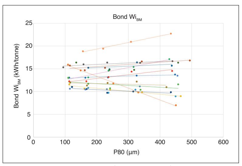
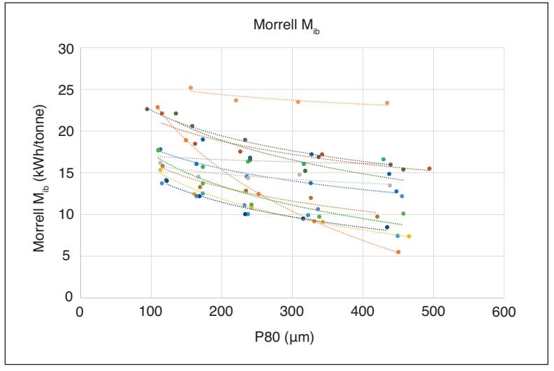
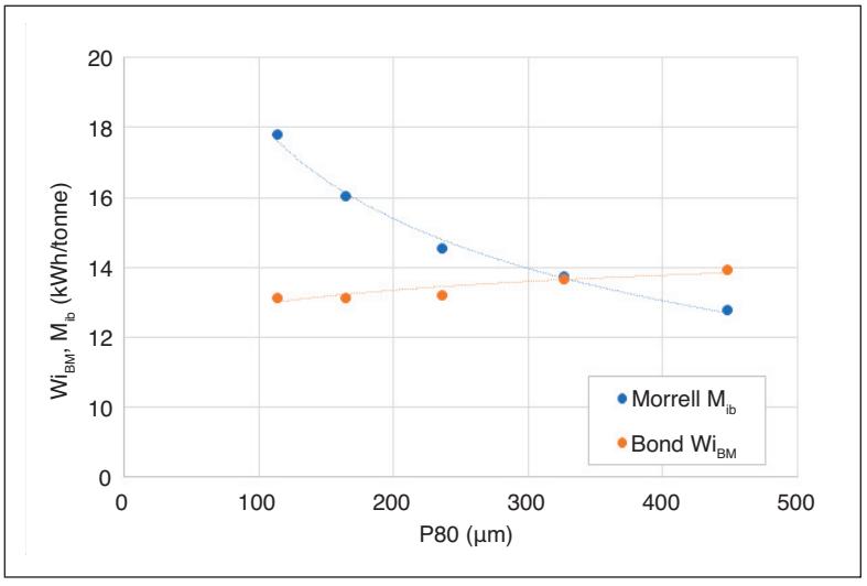
Bond (1959) published the full details of the laboratory ball work index tests on 14 different ore types. For each ore type, he repeated the test at five different grind sizes to determine how the various test parameters and the Bond ball work index varied with grind size. Figure 1 summarizes the resultant trends from his data and shows there is a wide spectrum of relationships, approximately half of which indicate that the Bond ball mill work index increases with decreasing grind size, and approximately half indicate the opposite. However, if all his data are aggregated, the results indicate that the average Bond ball work index is reasonably constant over the range of grind sizes he tested (Figure 3). Figure 2 shows the trends from the Mib values. In all cases, the Mib increases with decreasing grain sizes. If Bond's laboratory data are aggregated, then the average trend in Mib with grind size (Figure 3), is obtained. The equivalent trend in Bond's WiBM is also shown for comparison purposes. Although both Bond and Morrell recommend that the laboratory test should be carried out at the same (or similar) grind size to the plant, the consequences of not doing this are likely to be more significant when using the Mib and the Morrell equations.

To limit the impact of incorrect application of the Mib, the relationship shown in equation 1b was developed for cases where only a single Bond laboratory work index test has been done and it is required to apply the Mib in a situation which has a different grind size to the one that the laboratory test achieved. The exponent of 0.24 in this equation comes from fitting a power function to the trend in Figure 3.

$$ M_{ibtarget} = M_{ibref} \times \left( \frac{P80_{ref}}{P80_{target}} \right)^{0.24} $$ (1b)

Where:

Mibtarget is Mib in the calculation that is required to be carried out

Mibref is Mib obtained using the data from the Bond laboratory ball work index

P80target is P80 in the calculation that is required to be carried out

P80ref is P80 obtained in the Bond laboratory ball work index test

Worked example:

A Bond laboratory ball mill work index test was conducted using a closing screen of 150 μm which gave a P80 of 108 μm. A calculation is required to be carried out to estimate the specific energy required to reduce a feed generated by a particular upstream comminution circuit to a final product of 72 μm using a closed circuit ball mill.

Input data:

Mib calculated from the Bond test = 16.0 kWh/t

Reference P80 from the Bond test = 108 μm

Target P80 = 72 μm

Calculations:

From equation 1b:

$$ M_{\text{ibtarget}} = 16.0 \times \left(\frac{108}{72}\right)^{0.24} $$ $$ = 17.6 \text{ kWh/t} $$

5. MORRELL EQUATIONS

Given a circuit feed F80 and final product P80, plus the relevant hardness parameters, Morrell's equations can be used to predict the overall specific energy of most comminution circuit configurations. Full details of these equations are given in Annex B. However, they are all based on the same general energy-size reduction relationship represented by equation 2 (Morrell, 2004b). The following equations are made for a full circuit and cannot be broken down to assess the AG and/or ball mill efficiency individually.

$$ W = M_i \times 4 \times (x_2^{f(x_2)} - x_1^{f(x_1)}) $$ (2)

W is the specific comminution energy (kWh/t), Mi refers to hardness parameters (i.e., work index related to the breakage property of an ore) from SMC® and WiBM tests (kWh/t), x2 is 80% passing size for the product or the P80 (μm), x1 is the 80% passing size for the feed or the F80 (μm), and f(xj ) is defined as:

For tumbling mills, W relates to the power at the pinion or for gearless drives, the motor output. For HPGRs, W is the energy input to the rolls, whereas for conventional crushers, W relates to the specific energy as determined using the motor input power, less the no-load power.

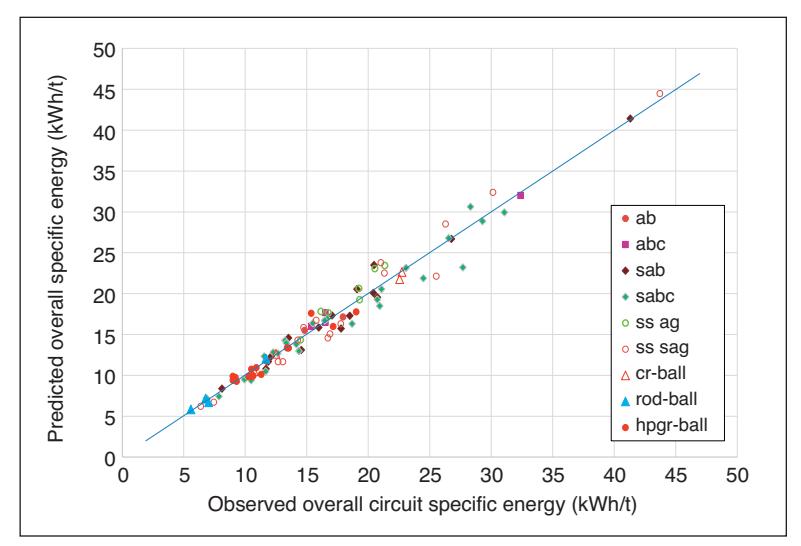
The equations above were developed with the aid of a database of 98 full data sets covering 74 operating plants treating more than 110 ore types. The database covers all of the most popular circuit configurations. The equations predict the overall specific energies of these plants with a high degree of accuracy (1 standard deviation is 7.0% of the relative errors). The observed and predicted specific energies of all of these circuits are plotted in Figure 4.

In Section 6, the equations are applied to three types of circuits to demonstrate their application to assessing the energy utilization of an existing plant. Annex C contains worked examples showing how these equations are used to predict the overall comminution circuit specific energy. The equations can also be found online on the SMC Testing web site (http://www.smctesting.com/tools) in the form of a free "tool" that enables the user to obtain the overall circuit specific energy of most common circuits, given the

relevant ore characterization values plus the F80 and P80 values.

6. USING THE MORRELL EQUATIONS

The data from the plant comprise a measured specific energy for the overall comminution circuit plus the F80 and P80 values. The SMC® and WiBM tests supply the relevant hardness parameters of the feed ore. These hardness parameters are used in a series of equations (Annexes B and C) that predict the expected specific energy of the same circuit, assuming it is well run as judged by the standards of circuits in the database used to develop the equations (Figure 4).

Assume that the existing plant, which has a semi-autogenous mill with pebble crushing followed by a ball mill (SABC circuit), was found to have an overall specific energy of 21.3 kWh/t. The measured feed size (F80) to the SAG mill was 100 mm and the measured ball mill cyclone overflow (P80) was 106 μm. SMC and WiBM tests on representative samples of the plant feed returned the following hardness parameters (in kWh/t):

Mia = 19.4

Mib = 18.8

Mic = 7.2

Mih = 13.9

Using these values in the relevant equations predicts that a well-run SABC circuit should consume on average 18.1 kWh/t to do the same duty as similar circuits from the database (see Annex C). The existing plant consumes 21.3 kWh/t, which is 18% more than predicted. Hence, the existing plant appears to be less efficient than expected. As mentioned in Section 5, for these equations, one standard deviation is 7.0% of the relative errors. The plant specific energy represents a difference of 2.6 standard deviations from the predicted value, which is highly significant (represents a situation that is expected to occur by chance with < 1% probability). Therefore, a detailed investigation of plant operations would be warranted to determine the causes of the inefficiency and how to correct them.

The above analysis enables effective benchmarking of the performance of a given operating circuit against similar circuits elsewhere and indicates the extent to which energy utilization efficiency could be improved—in this case potentially by as much as 18%. However, application of the equations can be further extended by comparing the performance of a given circuit with different circuit configurations. For example, using the ore characteristics and F80 and P80 values above, the specific energy of a crushing/ball milling circuit or crushing/HPGR/ball milling circuit can be predicted and compared with the specific energy for an SABC circuit.

With reference to the worked examples in Annex C, the expected specific energy for a crushing/ball mill circuit is 16.4 kWh/t (see Section C.3.6), which equates to an energy savings of 9% compared to a well-run SABC circuit and 23% compared to our (not so well-run) existing circuit. If the HPGR circuit is considered, it would be expected to require 14.8 kWh/t (see Section C2.5), which would give even greater energy savings. However, caution needs to be exercised because only the direct comminution machine energy requirements are considered in this analysis, and not ancillaries. Energy consumption tends to be higher for ancillaries in crushing/ball and HPGR/ball milling circuits than AG- and SAG-based circuits, and hence the overall operating power differences tend to be slightly less than indicated.

7. REFERENCES AND RECOMMENDED READING

Buckingham, L., Dupont, J.-F., Stieger, J., Blain, B., & Brits, C. (2011). Improving energy efficiency in Barrick grinding circuits. Proceedings of the 5th International Conference on Autogenous and Semiautogenous Grinding Technology (SAG 2011) . Montreal, QC: Canadian Institute of Mining, Metallurgy and Petroleum. 14 p.

Bond, F. C., (1959, February). Confirmation of the Third Theory, AIME Annual Meeting, San Francisco, California.

Doll, A. G. (2021). Mill motor power definitions. Revised August 26, 2021.

https://www.sagmilling.com/articles/1/view/?s=1

Global Mining Guidelines Group (GMG) (2016). Methods to survey an d sample grinding circuits for de termining energy efficiency. https://gmggroup.org/wp-

content/uploads/2016/05 /Guidelines_Surveying-and -Sampling-REV-2018.pdf

Global Mining Guidelines Group (GMG) (2021). Determining the Bond Efficiency of industria l grinding circuits.

https://gmggroup.org/wp-

content/uploads /2016/02/Guidelines_Bond-Efficienc y-REV-2018.pdf [link will be updated when 2021 version is published]

JKTech (2011). JK Drop Weight Tester. Retrieved on Septem ber 22, 2015, from

https://jktech.com.au/products/testing-equipment

Morrell, S. (2004a). Predicting the specific energy of autogenous and semi-autogenous mills from small diameter drill core samples. Minerals Engineering , 17(3), 447–451.

http://dx.doi.org/10.1016/j.mineng.2003.10.019

Morrell, S. (2004b). An alternative energy-size relationship to that proposed by Bond for the design and optimisation of grinding circuits. International Journal of Mineral Processing , 74(1–4), 133–141.

http://dx.doi.org/10.1016/j.minpro.2003.10.002

Morrell, S. (2006). Rock characterisation for high pressure grinding rolls circuit design. Proceedings of the International Autogenous and Semi Autogenous Grinding Technology Conference, Vol. IV (pp. 267–278).

Morrell, S. (2008). A method for predicting the specific energy requirement of comminution circuits and assessing their energy utilisation efficiency. Minerals Engineering, 21(3), 224–233.

http://dx.doi.org/10.1016/j.mineng.2007.10.001

Morrell, S. (2009). Predicting the overall specific energy requirement of crushing, high pressure grinding roll and tumbling mill circuits. Minerals Engineering , 22(6), 544–549.

http://dx.doi.org/10.1016/j.mineng.2009.01.005

Morrell, S. (2010). Predicting the specific energy required for size reduction of relatively coarse feeds in conventional crushers and high pressure grinding rolls. Minerals Engineering , 23(2), 151-153.

https://www.sciencedirec t.com/science/article/abs/ pii/S089268750900257X

SMC Testing Pty Ltd. (2021). The SMC Test® is the most widely-used comminution test in the world for AG & SAG Mills, HPGRs and Crushers. Retrieved on June 1, 2021, from http://www.smctesting.com/about

Stephenson, I. (1997). The downstream effects of high pressure grinding rolls processing. The University of Queensland .

Zervas, G. (2019). The Metcalf concentrator HRC™3000: Performance at variable specific force. Proceedings of an International conference on autogenous grinding, semi-autogenous grinding and high pressure grinding roll technology. Vancouver, BC, Canada.

ANNEX A: SMC TEST®

A.1 General Description

The SMC Test® (SMC Testing Pty Ltd., 2015) uses either crushed rock pieces that are very closely sized from sieving ("crush and select" method; Figure A1) or particles that are cut to similar size from a drill core using a diamond saw ("cut-core" method; Figure A2). The former method is used when samples are sourced from feed to an existing plant or sufficient drill core is available. The latter method is used when drill core sample availability is limited. Almost any drill core size is suitable, including cores that have been quartered (slivered). The chosen particles are broken using a closely controlled range of impact energies with the JKTech Drop Weight Tester (JKTech, 2011). The raw data from breakage at these energies are processed by SMC Testing Pty Ltd. via JKTech and generate the ore hardness parameters, Drop Weight index (DWi), Mia, Mic, and Mih, which are used in power-based equations, as well as the JKTech simulation parameters A, b, and ta. The specific gravity of the rock is also measured and reported.

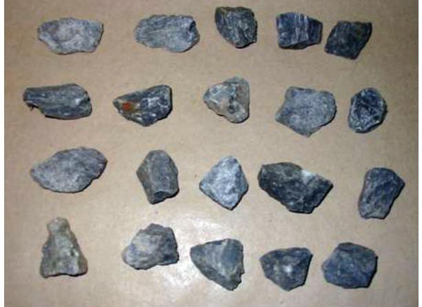
Figure A1. Particles Selected for SMC Testing from Crushed Rock Figure A2. Particles Selected for SMC Testing from Cutting a Drill Core

A.2 Sample Quantity

The amount of sample that is required depends on the rock sample source (e.g., crushed rock pieces vs. drill core, particle/core size, and whole vs. halved vs. quartered core), as well as the size fraction chosen to do the SMC Test® and whether the sample is going to be prepared by crushing or cutting. These factors are best discussed with the metallurgical laboratory at the planning stage. However, in the majority of cases, 15–20 kg of sample is more than enough to conduct a single test. It should be remembered that the SMC Test® products can be re-used for WiBM testing and the SMC Test® effectively being used as a feed preparation step for the WiBM test. If the sample source is from an existing mine in operation, then sample quantity should not be a problem. In such cases, it is far better to be generous when selecting the sample and take more than is normally required. Good practice is to take at least twice the amount required and to retain half the material in case problems necessitate rerunning the test.

SMC Tests® can be carried out on three size fractions, depending on the nature and quantity of the feed sample:

• –31.5+26.5 mm
• –22.4+19.0 mm
• –16.0+13.2 mm

If material quantity and size that is available for testing is no object (e.g., when the sample comes from an existing operation), then the –31.5 +26.5 mm fraction is recommended.

Formerly called "calibration," particle "size scaling" does not require size scaling to generate Mia, Mih, and Mic parameters from a SMC Test® because they are fixed functions of the DWi, which is produced as a standard output from the SMC Test®.

When the SMC Test® is used to estimate values of A and b (used in the JK AG/SAG mill model), a size scaling factor might be required. Since the average particle size used when testing with a JK drop-weight test is approximately 28– 30 mm, if the SMC Test is carried out on particles which are different sizes (e.g., size classes ranging from –22.4+19.0 mm or –16.0+13.2 mm), then a size scaling factor needs to be applied to account for the rock strength varying with particle size. However, if the SMC Test® is completed on particles with a similar size to 28—30 mm (i.e., from the –31.5+26.5 mm fraction), then the size scaling factor is not required. When size scaling is necessary, the required factors can be determined from analysis of the raw data from a relevant JK drop-weight test or, alternatively, can use SMC® Testing's extensive database with little to no loss in accuracy.

ANNEX B: MORRELL EQUATIONS

B.1 General Description

The Morrell approach divides comminution equipment into three categories:

• Tumbling mills (e.g., AG, SAG, rod, and ball mills)
• Conventional reciprocating crushers (e.g., jaw, gyratory, and cone)
• HPGRs

Tumbling mills are described using two work indices (Mia and Mib), whereas crushers and HPGRs each have one work index (Mic and Mih, respectively) (Morrell, 2008, 2009).

• Mia describes grinding of coarser material (P80 > 750 μm up to the P80 of the product of the last stage of crushing or HPGR size reduction prior to grinding) in tumbling mill circuit(s).
• Mib describes grinding of fine material (P80 < 750 μm down to P80 sizes typically reached by conventional ball milling, or approximately 45 μm) in tumbling mill circuit(s).
• Mic describes size reduction in crusher circuits.
• Mih describes size reduction in HPGR circuits.

Mia values are provided as a standard output from a SMC Test® (Morrell, 2008), whereas Mib values can be determined using the data generated by a conventional WiBM test (Mib is NOT the WiBM). Mic and Mih values are also provided as a standard output from a SMC Test® (Morrell, 2009).

For tumbling mills, Mia and Mib relate to coarse and fine ore properties, respectively. There is an additional efficiency factor that represents the influence of a pebble crusher in AG/SAG mill circuits. The choice of 750 μm as the division between "coarse" and "fine" particle sizes was determined during the development of the technique and was found to give the best overall results across the range of plants in the database. 750 μm is NOT the transfer size implicit in the approach is that distributions are parallel and linear in log-log space (see Section B.2.4). See equation 2 for the general size reduction equation from Morrell (2004b).

B.2 Specific Energy Determination for Comminution Circuits

The total specific energy (WT in kWh/t) to reduce in size the primary crusher product to the final product is given by:

$$ W_{T} = W_{a} + W_{b} + W_{c} + W_{h} + W_{s} $$ (B1)

Where Wa is the specific energy to grind coarser particles in tumbling mills, Wb is the specific energy to grind finer particles in tumbling mills, Wc is the specific energy for conventional crushing, Wh is the specific energy for HPGRs, and Ws is the specific energy correction for size distribution (all in kWh/t).

Only the W values associated with the relevant equipment in the circuit being studied are included in equation B1.

B.2.1 Tumbling Mills

To determine the specific energy to grind coarse particles (> 750 μm) in tumbling mills (Wa), equation 2 is written as:

$$ W_{a} = K_{1} \times M_{ia} \times 4 \times (x_{2}^{f(x_{2})} - x_{1}^{f(x_{1})}) $$ (B2)

Where:

Mia is the coarse ore work index (kWh/t), x2 is set to 750 μm, x1 is the F80 of the circuit feed, which is also the product of the last stage of crushing before grinding, f(xj ) is defined as:

K1 is the pebble crusher efficiency factor. The requirement for K1 arises from the fact that the energy efficiency of an AG/SAG mill circuit with a recycle pebble crusher is higher than a circuit without one. This is because the pebble crusher, which is inherently more energy efficient than a tumbling mill, does some of the comminution work that the tumbling mill would otherwise have to do and hence saves the tumbling mill energy. From empirical analysis the average energy saving is approximately 5% (and hence the average value of \( K_1 \) is 0.95), though it varies from circuit to circuit and typically falls in the range 0.9-1.0. Its magnitude depends on the amount of comminution work that the pebble crusher does and is related to the fraction of AG/SAG feed that reports to the pebble crusher (Peb_fr), the size of the pebbles fed to the crusher (F80_pc) and the size that the crusher reduces them to (P80_pc).

• Generally, if the number of pebbles is relatively large, then the pebble feed size will be relatively large, and this is the basis of the 0.95.
• If the crushing circuit is high-performing and if the number of pebbles is relatively large, the pebble feed size is relatively large and the pebble crusher product size is relatively small then the pebble crusher work will be maximized and K₁ will tend to 0.9 (or even lower in extreme cases).
• If information concerning how the pebble circuit is being operated is not available, then a reasonable assumption is to set K₁ to 0.95.
• If the pebble crusher circuit is doing little or no work, then there will be little or no energy saving in the SAG mill and hence K₁ will tend to unity and the SAG mill will behave as if it did not have a pebble crusher circuit.

Where relevant information concerning the pebble crusher circuit is available, then K₁ can be calculated as follows:

$$ K_1 = 1 - \frac{\left\{ \text{Peb}_{\text{fr}} \times S_c \times 1.19 \times \left( \text{P80}_{\text{pc}}^{\text{f(P80}_{\text{pc}})} - \text{F80}_{\text{pc}}^{\text{f(F80}_{\text{pc}})} \right) \right\}}{(750^{\text{f(750)}} - \text{F80}^{\text{f(F80)}})} $$ (B3)

Where:

Peb \( _{\rm fr} \) is the fraction of AG/SAG new feed that reports to the pebble crusher, F80 \( _{\rm pc} \) is the 80% passing size of the pebbles fed to the crusher, P80 \( _{\rm pc} \) is the 80% passing size of the pebble crusher product, S \( _{\rm c} \) is the coarse ore hardness parameter (see equation B10), 1.19 is the factor to account for the fact that the pebble crusher is in open circuit and F80 is the 80% passing size of the new feed to the SAG mill. As a rule of thumb Peb \( _{\rm fr} \) can be assumed to be 0.25, F80 \( _{\rm pc} \) can be estimated as 0.75 of the nominal pebble port apertures, and a reasonable assumption for P80 \( _{\rm pc} \) is 12-15mm.

Equation B3 was developed by considering that the specific energy of the pebble crusher ( \( W_{pc} \) ), expressed in terms of tonnes of new feed to the AG/SAG mill, is represented as follows:

$$ W_{pc} = Peb_{fr} \times S_c \times 1.19 \times M_{ic} \times 4 \times \left(P80_{pc}^{f(P80}pc) - F80_{pc}^{f(F80}pc)\right) $$ (B4)

If the tumbling mill had to do the same amount of size reduction on the pebble crusher feed, its specific energy expenditure \( (W_{tm,pc}) \) would be:

$$ W_{tmpc} = Peb_{fr} \times S_c \times 1.19 \times M_{ia} \times 4 \times (P80_{pc}^{f(P80_{pc})} - F80_{pc}^{f(F80_{pc})}) $$ (B5)

As the pebble crusher is doing the size reduction for the mill, then \( W_{tm,pc} \) is the energy that the pebble crusher saves the tumbling mill, thus improving its energy efficiency. Relative to a SAG mill with no pebble crusher ( \( K_1 \) =1) this can be expressed as:

relative energy saving = $$ \frac{W_{tm,pc}}{W_{a,K1=1}} $$ (B6)

Where \( W_{a,K1=1} \) is the specific energy to grind coarse particles (>750 ( \( \mu \) m)) in a SAG mill without a pebble crusher. \( K_1 \) is then defined as:

$$ K_1 = 1 - \left\{ \frac{W_{\text{tm,pc}}}{W_{\text{a,K1}=1}} \right\} $$ (B7)

See Tables B1 and B2 for a worked example for calculating the pebble crusher efficiency factor.

Table B1. Input Data, Pebble Crusher Efficiency Factor Worked Example

Input Data	Value
M ia	19.4 kWh/t
SAG new feed F80	100 mm
New feed rate to SAG mill	1,000 t/h
Pebbles crushing rate	250 t/h
Pebble crusher F80	52.5 mm
Pebble crusher P80	12.0 mm

Table B2. Calculations, Pebble Crusher Efficiency Factor Worked Example

$$ \text{Peb}_{\text{fr}} = \frac{250}{1,000} \\ = 0.25 \\ \text{K}_{1} \text{ from equation B3:} \\ \text{K}_{1} = 1 - \frac{\{ 0.25 \times 0.96 \times 1.19 \times ( 12,000 \stackrel{-(0.295 + \frac{12,000}{1,000,000})}{1,000,000} ) - 52,500 \stackrel{-(0.295 + \frac{52,000}{1,000,000})}{1,000,000} ) \}}{750 \stackrel{-}{-} ( 0.295 + \frac{750}{1,000,000} ) - 100,000 \stackrel{-}{-} ( 0.295 + \frac{100,000}{1,000,000} )}{1,000,000} ) \\ = 0.93 $$ $$ W_{a} \text{ from equation B2:} \\ W_{a} = 0.93 \times 19.4 \times 4 \times ( 750 \stackrel{-}{-} ( 0.295 + \frac{750}{1,000,000} ) - 100,000 \stackrel{-}{-} ( 0.295 + \frac{100,000}{1,000,000} ) )}{1,000,000} ) \\ = 0.93 \times 10.13 \text{ kWh/t $$ If there was no pebble crusher in the circuit, then K ₁ is set to 1 and W _a = 10.13 kWh/t

To determine the specific energy to grind fine particles (< 750 \( \mu \) m) in tumbling mills ( \( W_b \) ), equation 2 is written as:

$$ W_b = M_{ib} \times 4 \times (x_3^{f(x_3)} - x_2^{f(x_2)}) $$ (B8)

Where, \( M_{ib} \) is the fine material work index (kWh/t), \( x_3 \) is the P80 of the final grind ( \( \mu \) m), \( x_2 \) is set to 750 \( \mu \) m, \( f(x_j) \) is defined as:

The M_ib is calculated from data from the standard Wi_BM test using equation 1. Note that the Wi_BM test should be carried out with a closing screen mesh size that gives a final product P80 similar to that intended for the full-scale circuit. If the Wi_RM test was not carried out using the appropriate closing screen mesh size, then equation 1b should also be used in determining Mih.

Conventional Crushers B 2 2

To determine the specific energy for conventional crushing (W_c), equation 2 is written as:

$$ W_c = S_c \times K_2 \times M_{ic} \times 4 \times (x_2^{f(x_2)} - x_1^{f(x_1)}) $$ (B9)

Where, Sc is the coarse ore hardness parameter (see equation B10), K2 = 1.0 for crushers operating in closed circuit with a classifying screen, K2 = 1.19 for crushers operating in open circuit (e.g., pebble crusher in an AG/SAG circuit), Mic is the crushing ore work index provided directly by the SMC Test® (kWh/t), x2 is the P80 of the circuit product (μm), x1 is the F80 of the circuit feed μm, f(xj ) is defined as:

The parameter Sc accounts for the decrease in ore hardness that becomes significant in relatively coarse crushing applications such as primary, secondary, and pebble crushing circuits. In full-scale HPGR circuits—where feed sizes tend to be higher than those used in laboratory and pilot scale machines—the parameter has also been found to improve predictive accuracy (See Morrell [2010] Predicting the Specific Energy Required for Size Reduction of Relatively Coarse Feeds in Conventional Crushers and High Pressure Grinding Rolls, Technical Note). The parameter S is defined by the general equation B10:

Where, Ks is a machine-specific constant related to whether it is a conventional crushing circuit or an HPGR circuit (see Section B.2.3), x2 is the P80 of the circuit product (μm) and x1 is the F80 of the circuit feed (μm). In the case of conventional crushing circuits, Ks is set to 55 and the S parameter is referred to as Sc.

Sc should only be applied to a specific crushing circuit when it ranges between 0.5 to 1.0. If the calculation of Sc returns as a value greater than 1.0, then it should take the value of 1.0. If it returns as a value less than 0.5, then it should take the value of 0.5.

B.2.3 HPGRs

To determine the specific energy for HPGR size reduction (Wh), equation 2 is written as:

$$ W_{h} = S_{h} \times K_{3} \times K_{4} \times M_{ih} \times 4 \times (x_{2}^{f(x_{2})} - x_{1}^{f(x_{1})}) $$ (B11)

Where, Sh is the coarse ore hardness parameter used in HPGRs (substitute S with Sh in equation B10, with Ks set to 35), K3 = 1.0 for HPGRs operating in closed circuit with a classifying screen, K3 = 1.19 for HPGRs operating in open circuit, K4 is the specific grinding force efficiency factor (see equation B12), Mih is the ore paramater provided directly by the SMC Test® (kWh/t), x2 is the P80 of the circuit product (μm), x1 is the F80 of the circuit feed (μm), f(xj ) is defined as:

Sh should only be applied in a given HPGR circuit if it is in the 0.5 to 1.0 range. If the calculation of Sh returns a value greater than 1.0, it should take the value of 1.0. If it returns a value less than 0.5, it should take the value of 0.5.

The K4 term in equation B11 is required because the energy efficiency of HPGRs is dependent on the applied specific grinding force. K4 is defined as follows:

$$ K_4 = \frac{0.71 \times e^{(0.28 \times SF)}}{M_{ih}^{0.23}} $$ (B12)

Where SF is the applied specific grinding force in N/mm2.

The effect of K4 is to predict an increase in the required specific energy to achieve a certain size reduction as the applied specific force is increased, i.e., the HPGR size reduction efficiency apparently reduces as the applied specific force increases.

Whereas this might be true across the HPGR circuit, Ian Stephenson's 1997 PhD thesis "The Downstream Effects of High Pressure Grinding Rolls Processing" showed that in most cases, as the applied specific grinding force increased, the Bond laboratory ball work index of the HPGR product decreased in line with the degree of microcracking that he observed under an electron microscope. Hence, although the HPGR energy expenditure to achieve a given size reduction increases as the applied specific force increases, it is not necessarily wasted but instead helps save energy in the ball mill circuit. However, it is not yet clear what the effect is on the overall comminution circuit specific energy. Overall effects are likely to be small, therefore detecting them via plant performance data will be extremely challenging, if not impossible.

B.2.4 Specific Energy Correction for Size Distribution (Ws)

The approach described in this guideline assumes that the feed and product size distributions are parallel and linear in log-log space. If they are not, corrections are required. These corrections are most likely to be necessary in circuits where closed circuit secondary/tertiary crushing is followed by ball milling, because such crushing circuits tend to produce a product size distribution that is relatively steep compared to the ball mill circuit cyclone overflow. This is illustrated in Figure B1, which shows measured distributions from an open and closed crusher circuit, as well as a ball mill cyclone overflow. The closed circuit crusher distribution is steeper than the open circuit crusher distribution and ball mill cyclone overflow. Also, the open circuit distribution more closely follows the gradient of the cyclone overflow.

If a ball mill circuit was fed two distributions, each with the same P80, but with the open and closed circuit gradients in

Figure B1, the closed circuit distribution would require more energy to grind to the final P80. How much more energy is difficult to determine. However, it has been assumed that the additional specific energy for ball milling is the same as the difference in specific energy between open and closed crushing to reach the nominated ball mill feed size. The crusher is assumed to provide this energy. However, the ball mill has to supply this energy, and it has a higher work index than the crusher (i.e., the ball mill is less energy efficient than a crusher and has to input more energy to do the same amount of size reduction). Hence from equation B9, to crush to the ball mill circuit feed size (x2) in open circuit requires specific energy equivalent to:

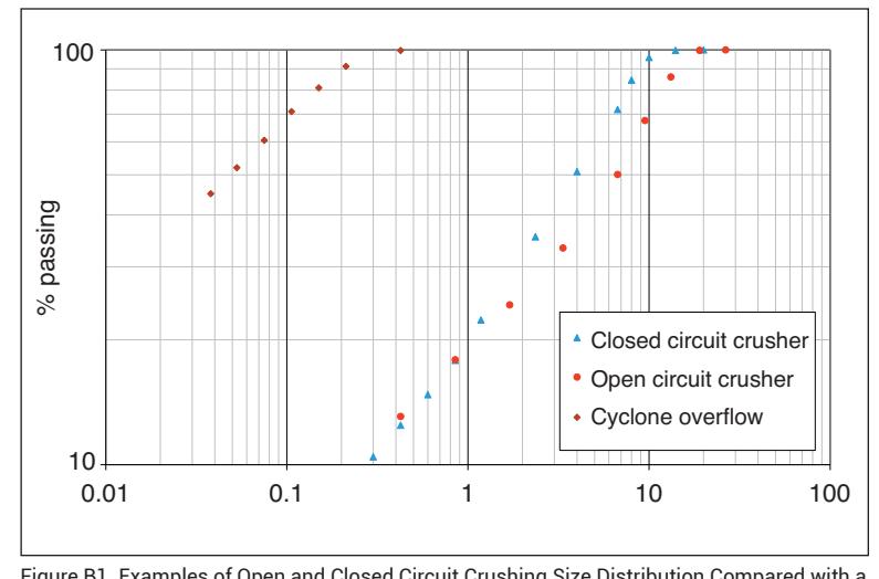
Figure B1. Examples of Open and Closed Circuit Crushing Size Distribution Compared with a Typical Ball Mill Cyclone Overflow Distribution

And from equation B9, to crush to the ball mill circuit feed size (x2) in closed circuit requires specific energy equivalent to:

The energy difference between the two equations above has to be provided by the milling circuit, allowing for the fact that the ball mill—with its lower energy efficiency—has to provide the energy, not the crusher. This energy is the Ws (equation B1) and for the above example is represented by:

Note that Mic from the previous two equations has been replaced with Mia, the coarse particle tumbling mill grinding work index. Also, Sc was set to unity because typically a tertiary crushing stage feeds the ball mill; Sc takes the value of 1 under these circumstances.

In AG/SAG-based circuits, Ws appears to be unnecessary. Product distributions in primary crusher feeds often have the shape shown in Figure B2, which has a very similar gradient to typical ball mill cyclone overflows.

A similar situation appears to apply with HPGR product size distributions (Figure B3). Interestingly, the data show that for HPGRs, closed circuit operation appears to require a lower specific energy to reach the same P80 as open circuit operation, even though the distributions for open and closed circuit appear to have almost identical gradients. Closer examination of the distributions shows that in closed circuit, the final product tends to have slightly less very fine material, which could account for the different energy requirements between the two modes of operation. It is also possible that recycled material in closed circuit is inherently weaker than new feed, because it has already passed through the HPGR and could have sustained micro-cracking.

A reduction in the WiBM as measured by testing HPGR products (compared it to the WiBM of HPGR feed) has been detected in many

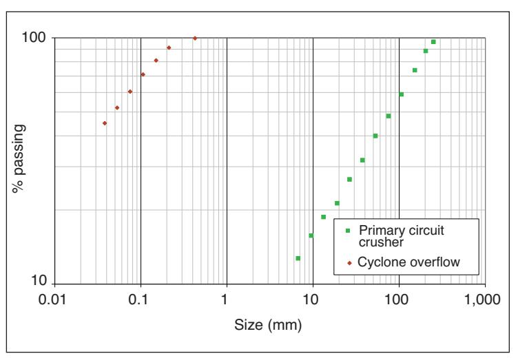
Figure B2. Example of a Typical Primary Crusher (Open Circuit) Product Size Distribution Compared with a Typical Ball Mill Cyclone Overflow Size Distribution

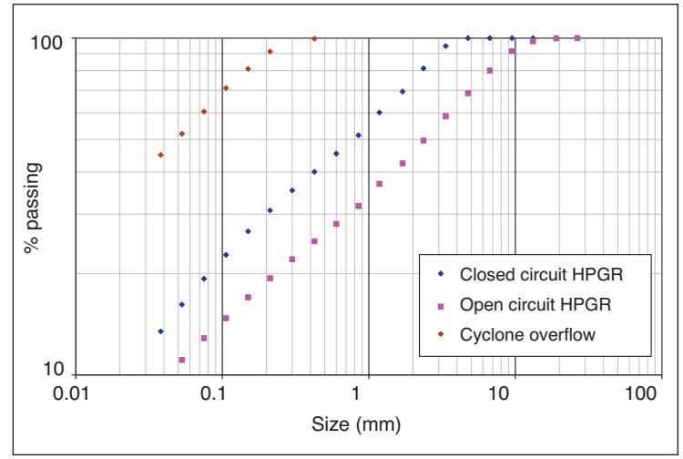
Figure B3. Examples of Open and Closed Circuit HPGR Size Distributions Compared with a Typical Ball Mill Cyclone Overflow Size Distribution cases in the laboratory (see Section B.2.5), and hence there is no reason to expect the same phenomenon would not affect the recycled HPGR screen oversize.

It follows from the above arguments that in HPGR circuits, which are typically fed with material from closed circuit secondary crushers, a similar feed size distribution correction should be applied. However, as the secondary crushing circuit uses little energy relative to the rest of the circuit (because it crushes to a relatively coarse size), the magnitude of size distribution correction is very small indeed—much smaller than the error associated with the technique—and hence may be omitted in calculations.

B.2.5 Weakening of HPGR Products

Various researchers have reported experimental laboratory results showing that the WiBM is lower for HPGR products than feed. The magnitude of this reduction varies with both the material type and the pressing force used but is typically < 10%. If HPGR products are available to conduct WiBM tests, then Mib values obtained from such tests can be used in equation B8. Alternatively, the Mib values from WiBM tests on HPGR feed material can be reduced by an amount that the user thinks is appropriate. Until more data become available from full-scale HPGR/ball mill circuits, it is suggested that, in the absence of WiBM data on HPGR product, the Mib results from HPGR feed material are reduced by 5-7% to allow for the effects of micro-cracking.

B.3 Validation

B.3.1 Tumbling Mill Circuits

The approach described in Section B.2 was applied to 98 industrial data sets (Figure B4). In all cases, the specific energy relates to the tumbling mills contributing to size reduction from the product of the final stage of crushing to the final grind. Data are presented in terms of equivalent specific energy at the pinion. It was assumed that power at the pinion was 93.5% of the measured gross (motor input) power, this value being typical of what is normally accepted to represent losses across the motor and gearbox. For gearless drives (socalled wrap-around motors) a value of 97% was used.

B.3.2 Conventional Crushers

Validation of equation 2 used 12 crushing circuits (25 data sets), including secondary, tertiary, and pebble crushers in AG/SAG circuits. Observed vs. predicted specific energies are given in Figure B5. The observed specific energies were calculated from the crusher throughput and the net power draw of the crusher as defined by:

Net power = Motor input power ‒ No-load power (B13)

No-load power tends to be relatively high in conventional crushers and hence net power is significantly lower than the motor input power. Examination of the 25 crusher data sets showed the motor input power was on average 20% higher than the net power.

B.3.3 HPGRs

Validation of equation 2 for HPGRs used data from 17 pilot and full-scale circuits (22 datasets), including those of Morenci and Tropicana. The specific grinding force range of these circuits was 1.8–5.3 N/mm2. The data relate to net specific energy using the assumption that energy losses across the motor and gearbox amounted to approximately 10%. On the basis of these data the indicated accuracy is as illustrated in Figure B6. The standard deviation of the relative error is 6.3%.

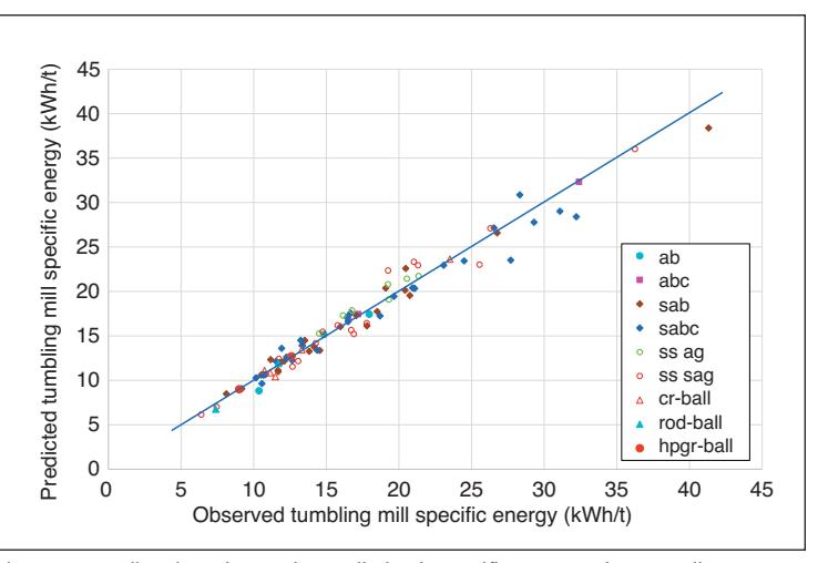
Figure B4. Predicted vs Observed Overall Circuit Specific Energy using Morrell's Equations. Note: a = autogenous; b = ball mill; c or cr = crushing; g = grinding; sa = semiautogenous; sabc = semi-autogenous mill with pebble crushing, followed by a ball mill; ss = single-stage.

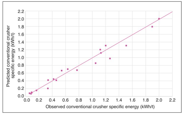
Figure B5. Predicted vs. Observed Conventional Crusher Specific Energy

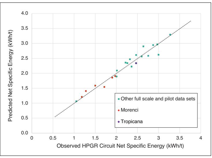
Figure B.6 Predicted vs. Observed HPGR Circuit Specific Energy

ANNEX C: WORKED EXAMPLES

The goal is to estimate the overall specific grinding energy to reduce a primary crusher product with a P80 of 100 mm to a final product P80 of 106 μm. SMC and WiBM tests were carried out on a representative ore sample (Table C1).

Three circuits are evaluated: SABC, HPGR/ball mill, and conventional crushing/ball mill.

Table C1. Values Used for Specific Grinding Energy Calculations

Parameter	Value (kWh/t)	Test
Mia	19.4	SMC
Mib	18.8	WiBM
Mic	7.2	SMC
Mih	13.9	SMC

C.1 SABC Circuit

C.1.1 Coarse Particle Tumbling Mill Specific Energy

Using equation B2 from Annex B:

$$ W_{a} = K_{1} \times 19.4 \times 4 \times \left(750^{-\left[0.295 + \frac{750}{1,000,000}\right]} - 100,000^{-\left[0.295 + \frac{100,000}{1,000,000}\right]}\right) $$ $$ = K_{1} \times 10.13 \text{ kWh/t} $$

Assuming that 25% of new feed reports to the pebble crushing circuit, the pebble crusher feed F80 is 52.5 mm and the product P80 is 12 mm then using equation B3 from Annex B:

$$ K_{1} = 1 - \frac{\{0.25 \times 0.96 \times 1.19 \times (12,000^{-(0.295 + \frac{12,000}{1,000,000})} - 52,500^{-(0.295 + \frac{52,500}{1,000,000})}\}\} - 52,500^{-(0.295 + \frac{52,500}{1,000,000})}\}\}}{\,} $$ $$ = 0.93 $$ $$ W_{a} = 0.93 \times 10.13 \text{ kWh/t} $$ $$ = 9.4 $$

C.1.2 Fine Particle Tumbling Mill Specific Energy

Using equation B8 from Annex B:

$$ W_{b} = 18.8 \times 4 \times \left(106^{-\left(0.295 + \frac{106}{1,000,000}\right)} - 750^{-\left(0.295 + \frac{750}{1,000,000}\right)}\right) $$ $$ = 8.4 \text{ kWh/t} $$

C.1.3 Pebble Crusher Specific Energy

In this circuit, the pebble crusher feed F80 is assumed to be 52.5 mm. As a rule of thumb, this value can be estimated as 0.75 of the nominal pebble port aperture (in this case the pebble port aperture is 70 mm). The pebble crusher is set to give a product P80 of 12 mm. The pebble crusher feed rate is expected to be 25% of new feed rate.

Using equations B9 and B10 from Annex B:

$$ W_c = 55 \times (12,000 \times 52,500)^{-0.2} \times 1.19 \times 7.2 \times 4 \times \left(12,000^{-\left(0.295 + \frac{12,000}{1,000,000}\right)} - 52,500^{-\left(0.295 + \frac{52,500}{1,000,000}\right)}\right) $$ $$ = 1.08 \text{ kWh/t} $$

The product of this calculation is 1.08 kWh/t when expressed in terms of the crusher feed rate. It is 0.3 kWh/t (1.08 × 0.25) when expressed in terms of the SABC circuit new feed rate.

Note that in this case, Sc = 55 × (12,000 × 52,500)–0.2 = 0.96.

C.1.4 Total Net Comminution Specific Energy

Using equation B1 from Annex B:

C.2 HPGR/Ball Mill Circuit

In this circuit, primary crusher product is reduced to a HPGR circuit feed P80 of 35 mm by closed circuit secondary crushing. The HPGR is also in closed circuit and reduces the 35 mm feed to a circuit product P80 of 4 mm. This product is then fed to a closed circuit ball mill, which takes the grind down to a P80 of 106 μm.

C.2.1 Secondary Crushing Specific Energy

Combining equations B9 and B10 from Annex B:

$$ W_{c} = 55 \times (35,000 \times 100,000)^{-0.2} \times 1 \times 7.2 \times 4 $$ $$ \times \left(35,000^{-\left(0.295 + \frac{35,000}{1,000,000}\right)} - 100,000^{-\left(0.295 + \frac{100,000}{1,000,000}\right)}\right) $$ $$ = 0.4 \text{ kWh/t} $$

C.2.2 HPGR Specific Energy

Combining equations B10 and B11 from Annex B:

$$ W_{h} = 35 \times (4,000 \times 35,000)^{-0.2} \times 1 \times K_{4} \times 13.9 \times 4 $$ $$ \times \left(4,000^{-\left(0.295 + \frac{4,000}{1,000,000}\right)} - 35,000^{-\left(0.295 + \frac{35,000}{1,000,000}\right)}\right) $$ $$ = K_{4} \times 2.4 \text{ kWh/t} $$

Assuming the HPGR will be operated with an applied specific grinding force of 3.0 N/mm2, then using equation B12 from Annex B:

Hence:

$$ W_{h} = 0.9 \times 2.4 \text{ kWh/t} $$ $$ = 2.2 \text{ kWh/t} $$

C.2.3 Coarse Particle Tumbling Mill Specific Energy

Using equation B2 from Annex B:

C.2.4 Fine Particle Tumbling Mill Specific Energy

Using equation B8 from Annex B:

Note that in this case, the effects of micro-cracking were assumed to soften the ore by 5% for the coarse (Wa) and fine (Wb) fractions of the tumbling ball mill.

C.2.5 Total Net Comminution Specific Energy

Using equation B1 from Annex B: $$ W_t = 0.4 + 2.2 + 4.2 + 8.0 = 14.8 \text{ kWh/t} $$

C.3 Conventional Crushing/Ball Mill Circuit

In this circuit, primary crusher product is initially reduced in size to a P80 of 35 mm in an open circuit secondary crusher. This material is then reduced in size to a P80 of 6.5 mm via a closed tertiary/quaternary crushing circuit. This product is then fed to a closed circuit ball mill, which grinds to a P80 of 106 μm.

C.3.1 Secondary Crushing Specific Energy

Combining equations B9 and B10 from Annex B:

$$ W_{c} = 55 \times (35,000 \times 100,000)^{-0.2} \times 1.19 \times 7.2 \times 4 \times \left(35,000^{-\left(0.295 + \frac{35,000}{1,000,000}\right)} - 100,000^{-\left(0.295 + \frac{100,000}{1,000,000}\right)}\right) $$ $$ = 0.5 \text{ kWh/t} $$

C.3.2 Tertiary/Quaternary Crushing Specific Energy

Combining equations B9 and B10 from Annex B:

Note that in this case, Sc = 55 × (6,500 × 35,000)–0.2 = 1.17. Because it is greater than unity, Sc does not apply and is set to 1.

C.3.3 Coarse Particle Tumbling Mill Specific Energy

Using equation B2 from Annex B:

$$ W_{a} = 1 \times 19.4 \times 4 \times \left(750^{-\left(0.295 + \frac{750}{1,000,000}\right)} - 6,500^{-\left(0.295 + \frac{6,500}{1,000,000}\right)}\right) $$ $$ = 5.5 \text{ kWh/t} $$

C.3.4 Fine Particle Tumbling Mill Specific Energy

Using equation B8 from Annex B:

$$ W_b = 18.8 \times 4 \times \left(106^{-\left(0.295 + \frac{106}{1,000,000}\right)} - 750^{-\left(0.295 + \frac{750}{1,000,000}\right)}\right) $$ $$ = 8.4 \text{ kWh/t} $$

C.3.5 Size Distribution Correction

Please refer to Section B.2.4 from Annex B for more information:

$$ W_s = 0.19 \times 19.4 \times 4 \times (6,500^{-\left(0.295 + \frac{6,500}{1,000,000}\right)} - 100,000^{-\left(0.295 + \frac{100,000}{1,000,000}\right)}) $$ $$ = 0.9 \text{ kWh/t} $$

C.3.6 Total Net Comminution Specific Energy

Using equation B1 from Annex B:

ANNEX D: ESTIMATING THE Mib FROM THE Wi BM AND CLOSING SCREEN SIZE

If full details of the Bond laboratory work index test are not available to determine the Mib, it is possible to estimate the required data if the WiBM and the closing screen size are known. This is done by rearranging Bond's WiBM equation D1 and using the fact that the P80 is typically 0.76 of the P100 and that the F80 is, on average, 2,250 μm. As a result, the Gpb can be estimated using equation D2 and subsequently used in equation D3, to estimate the Mib.

$$ Wi_{BM} = \frac{49.05}{P100^{0.23} \times (Gpb)^{0.82} \times 10 \times \left(\frac{1}{\sqrt{P80}} - \frac{1}{\sqrt{F80}}\right)} $$ (D1)

$$ Gpb_{(estimated)} = \left\{ \frac{4.9}{P100^{0.23} \times Wi_{BM} \times \left( \frac{1}{\sqrt{0.76 \times P100}} - \frac{1}{\sqrt{2,250}} \right)} \right\}^{\left( \frac{1}{0.82} \right)} $$ (D2)

$$ M_{ib} = \frac{18.18}{P100^{0.295} \times Gpb_{(estimated)} \times ((0.76 \times P100)^{f(0.76 \times P100)} - 2,250^{f(2,250)})} $$ (D3)